The correlation coefficient in the qqplot can be used as a test for normality (in the case of a normal qqplot, or for some other null distribution model). See for instance this paper Developing a Test of Normality in the Classroom.
But if the correlation in the plot is useful as an effect size, is another matter ... test statistics by themselves are not necessarily useful as an effect size, it is better to start with an estimator of some parameter, but in this case of goodness of fit testing, which parameter?
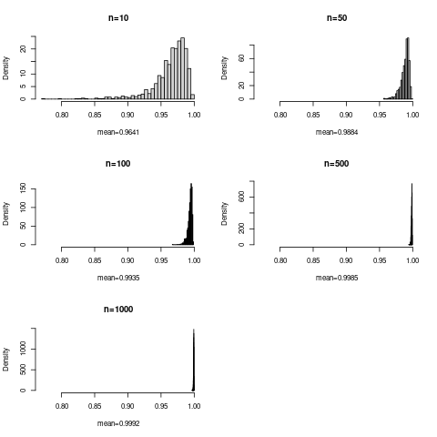
The rest is a long comment to some of the OP comments above: Let us do some simulation in the case of the normal distribution, so tests of normality. Below is a plot of simulation with 1000 replications and various sample sizes:

The OP noted that means increase with sample size. The plot shows the reason, there is a hard upper limit at 1, but a long lower tail, especially with lower sample size. So the histograms do not have the same form, they are skew for low $n$ and more symmetric for higher $n$. This in itself shows that the correlation cannot be a good measure of effect size.
For reference, below the R code used:
simcor <- function(N,  R,  simfun=rnorm, qfun=qnorm,  ...) { # N can be a vector
    res <- numeric(length=length(N))
    corrs <- matrix(as.numeric(NA), R, length(N))
    colnames(corrs) <- paste0("n=", N)
    for (i in seq_along(N)) {n <- N[i]
        vals <- matrix( simfun(n*R, ...), R, n)
        mean_corrs <- numeric(R)
        pp <- ppoints(n)  ;   qq <- qfun(pp, ...)
        for (r in 1:R) {
            samp <- vals[r, , drop=TRUE]
            mean_corrs[r] <- cor(sort(samp), qq)
        }
        res[i] <- mean(mean_corrs) ; names(res) <- N
        corrs[, i] <- mean_corrs
    }
    return(list(mean_corr=res,  corr=corrs))
}

run_norm <- simcor(c(10, 50, 100, 500, 1000),  1000)

xran <- c(0.77, 1)

 opar <-  par(mfrow=c(3, 2))
 for (i in seq_along(run_norm[[1]])) {
     hist(run_norm[[2]][, i], "FD", prob=TRUE, main=colnames(run_norm[[2]])[i],
          xlab=paste0("mean=", round(run_norm[[1]][i], 4)),
          xlim=xran) }
par(opar)

