Bootstrap for random effects logistic regression to get CI for difference in proportions

Question

Let's say I have two observations of a binary variable per patient on two different treatments for a sensible number of patients, some variable like age, and I'm fitting a model like this in R:

library(lme4)
library(tidyverse)

logit = function(x) log(x) - log1p(-x)
inv.logit = function(x) exp(x)/(1+exp(x))

set.seed(1234)
example = tibble(patient=rep(1:100, each=2), 
                 randeff = rep(rnorm(100), each=2),
                 treatment=rep(0:1, 100),
                 age = rep(exp(3+rnorm(100)), each=2),
                 logitprob = logit(0.7) + treatment - age/80 + randeff,
                 responder = rbinom(n=200, 
                                    size=1, 
                                    prob=inv.logit(logitprob)))

fit1 = glmer(data=example,
             responder ~ (1|patient) + treatment + age, 
             family=binomial(link="logit"))

summary(fit1)

What do I want?

What I'd like to do now, is to estimate a difference in the responder proportion between the treatments and get a confidence interval for that. Obviously, this has two complications: 1) I need to account for the random effects and 2) I want to account for the age covariate. I.e. assuming that this is a reasonably representative sample from the population, I'd guess I'd want predictions for a covariate distribution that is the empirical distribution I observed - if there's a better/more logical way of approaching this, then I'm interested in that, too.

I'd have thought in the example the estimate should not be too far away from 0.22 (on my machine with these random number seeds, I got 0.69 and 0.47 as the mean proportions):

example %>%
  group_by(treatment) %>%
  summarize(mean(responder))

Point estimate

Obviously, I can get predicted logits from this model and apply the inverse-logit to these to get probabilities and form their difference within patient and then average. That would seem like a sensible point estimate.

Option 1: Confidence interval via non-parametric bootstrapping

It occured to me that boostrapping would be one way of doing this:

• To respect the correlations in the data, I presumably need to bootstrap patients (rather than records).
• For each bootstrap sample I fit the model.
• For each fitted model, I predict for the bootstrap sample it was fitted to.
• Then I calculate the point estimate as above

However, what do I do, when I have the same patient repeatedly in the data? My initial guess is that I should treat that as separate levels of patient. I.e. if my bootstrap sample includes patient 1 ten times, I should turn that into patient 1a, 1b, ..., 1j that each get their own random intercept effect. Example code:

library(boot)
fit_glmm_on_bootstrap <- function(original, indices) {
  patients = original[indices]
  tmp_data = map2(patients, 1:length(patients),
                  function(x,y) example %>% filter(patient==x) %>% mutate(new_id=y)) %>%
    bind_rows()
  
  tmp_model = glmer(data=tmp_data,
                    formula = responder ~ (1|new_id) + treatment + age,
                    family=binomial(link="logit"))
  (tmp_data %>%
      mutate(preds = inv.logit(predict(tmp_model, newdata=tmp_data)),
             preds = ifelse(treatment==0, -preds, preds)) %>%
      group_by(new_id) %>%
      summarize(difference = sum(preds)) %>%
      ungroup() %>%
      summarize(difference=mean(difference))
  )$difference
}

booted = boot(data = unique(example$patient),
              statistic = fit_glmm_on_bootstrap, 
              R=999, stype="i", sim="ordinary")

Is that correct?

At least with a small dummy dataset, I'm getting a bit of trouble with convergence warnings (e.g. boundary (singular) fit: see ?isSingular) on some of the bootstrap samples.

Option 2: Using bootMer

The alternative I looked at was using the lme4::bootMer function (which the lme4 documentation seems to suggest could do something like this), perhaps like this:

bootres = bootMer(x = fit1, type = "parametric",
        FUN = function(x) {
          (example %>%
             mutate(preds = inv.logit(predict(object=x, newdata=example, re.form=NULL)),
                    preds = ifelse(treatment==0, -preds, preds)) %>%
             group_by(patient) %>%
             summarize(difference = sum(preds)) %>%
             ungroup() %>%
             summarize(difference = mean(difference)))$difference },
        nsim=999)

boot.ci(bootres, type=c("norm", "basic", "perc"))
# That gets me:
# Intervals : 
# Level      Normal              Basic              Percentile     
# 95%   ( 0.0663,  0.3058 )   ( 0.0647,  0.3052 )   ( 0.0628,  0.3032 )  

However, I'm a bit uncertain what this function does on the inside (esp. with respect to the random effects and e.g. whether "parametric" is a good choice, if I'm willing to "believe" in my model) and whether this will do something sensible. Does someone have experience on this?

Option 3: Bayesian random effects model

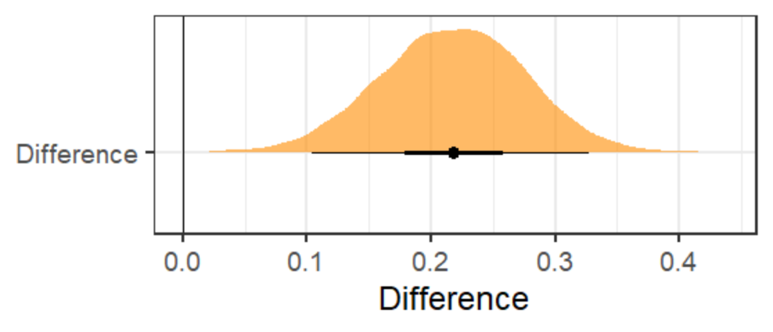
This is following Frank Harrell's suggestion in a comment and seems to behave about as expected (unsurprising, we know Bayesian models really make it easy to do inference on transformations of model parameters). I think I can justify these priors, but I'd still be interested on how to properly implement a purely frequentist alternative.

library(rstanarm)
library(tidybayes)
bayes_model = stan_glmer(data=example %>% mutate(age = scale(age)),
                    formula = responder ~ (1|patient) + treatment + age,
                    family=binomial(link="logit"),
                    prior_intercept = normal(scale=3.1416, autoscale=FALSE), # Approximately Beta(0.5, 0.5) prior if all for probability, if all other terms zero
                    prior_covariance = decov(shape = 1, scale = 4), # Exponential(rate=0.25) prior on hierarchical scale parameter
                    prior = normal(scale=3.1416, autoscale=FALSE))

posterior_for_difference = example %>% 
  mutate(record=1:n()) %>%
  left_join(
    as_tibble(t(inv.logit(posterior_linpred(object = bayes_model, 
                                            newdata=example %>% mutate(age = scale(age)), 
                                            re.form=NULL))),
              .name_repair= ~ vctrs::vec_as_names(..., repair = "unique", quiet = TRUE)) %>%
      mutate(record=1:n()), 
    by = "record") %>%
  pivot_longer(cols=`...1`:`...4000`, names_to="m", values_to="resp") %>%
  group_by(m, treatment) %>%
  summarize(mean_resp = mean(resp), .groups="drop") %>%
  pivot_wider(id_cols="m", values_from="mean_resp", names_from="treatment") %>%
  mutate(Difference = `1`-`0`)

posterior_for_difference %>%
  summarize(median_qi(Difference))
# This got me:
#       y  ymin  ymax .width .point .interval
#    <dbl> <dbl> <dbl>  <dbl> <chr>  <chr>    
#  1 0.218 0.104 0.328   0.95 median qi  

posterior_for_difference %>%
  ggplot(aes(x=Difference, y="Difference")) +
  theme_bw(base_size=18) +
  theme(axis.title.y=element_blank()) +
  geom_vline(xintercept=0) +
  stat_halfeyeh(.width = c(0.5, 0.95), slab_alpha=0.6, fill="darkorange")

The main question I have for the Bayesian approach is: should I simulate a new population (random effects randomly drawn, covariates distribution using the observed distribution) or - as I did - sample from the fitted random effects?!

Answer 1

More of an extended set of comments than an answer.

The bootMer() and its associated simulate.merMod() functions in lme4 contain hints as to what works in practice whether in frequentist or Bayesian modeling. (The package doesn't seem to contain functions for case resampling; more on that later.) Quotes below are from the manual page for bootMer().

The use.u parameter determines whether the random effects (u) are used at their estimated values (use.u = TRUE) or simulation/sampling is done from the "spherical" random effects (use.u = FALSE). According to the bootMer() manual page, "resampling from the estimated values of u is not good practice."* That would argue against resampling from your fitted random effects, whether in Bayesian or frequentist modeling.

The type setting determines how errors/responses are sampled. With type = "parametric", "the i.i.d. errors (or, for GLMMs, response values drawn from the appropriate distributions) are resampled." With type = "semiparametric":

the i.i.d. errors are sampled from the distribution of (response) residuals. (For GLMMs, the resulting sample will no longer have the same properties as the original sample, and the method may not make sense; a warning is generated.)

As this question is about a logistic model, the "semiparametric" setting would thus be unwise.

So with bootMer() and a logistic model you would use type = "parametric", thus sampling response values drawn from the underlying binomial distribution. Your choice is whether to use random-effect values fixed at their estimates (use.u = TRUE) or to sample from the estimated distribution of random-effect values (use.u = FALSE). The former choice would seem to make your results conditional on your sample.

With respect to case resampling, Michael Chernick notes that: "The nonparametric bootstrap has been shown to be more robust than the parametric bootstrap when the model is misspecified." That said, it's not clear to me how to deal correctly with resamples that don't seem to be fit properly. If it's just a matter of slow convergence that might be handled by altering fitting options, but if a fit to a resample is really impossible then omitting those resamples would seem to lead to a bias.

As the Bayesian model seems to work well, I suspect that you will stick with that. The warning about resampling from fitted fixed effects in the bootMer() manual page would suggest you should move to drawing from their distribution instead.

---

*The citation on this point in the manual page is to: Morris, J. S. (2002). The BLUPs Are Not ‘best’ When It Comes to Bootstrapping. Statistics & Probability Letters 56(4): 425–430. doi:10.1016/S0167-7152(02)00041-X. I haven't read that myself.