2
$\begingroup$

I have a question about priors and likelihoods and their visualisation.

A Bernoulli likelihood is $$\theta^{N_1}(1 - \theta)^{N_0}$$ where $N_1$ and $N_0$ are number of success and failures, respectively.

I want to visualise (in R) a conjugate Beta prior $Beta(2, 2)$ and Likelihood:

N_1 = 4
N_0 = 1

N = N_1 + N_0

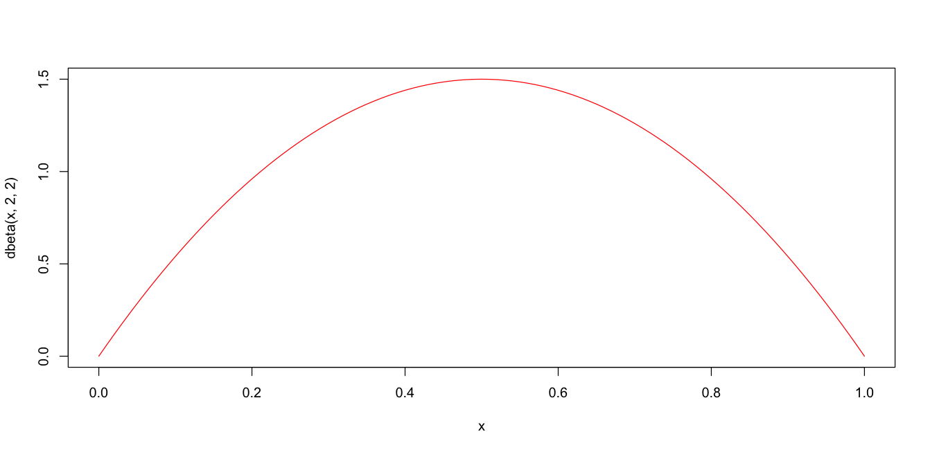
curve(dbeta(x, 2, 2),
      col = 'red')

Prior Beta(2, 2)

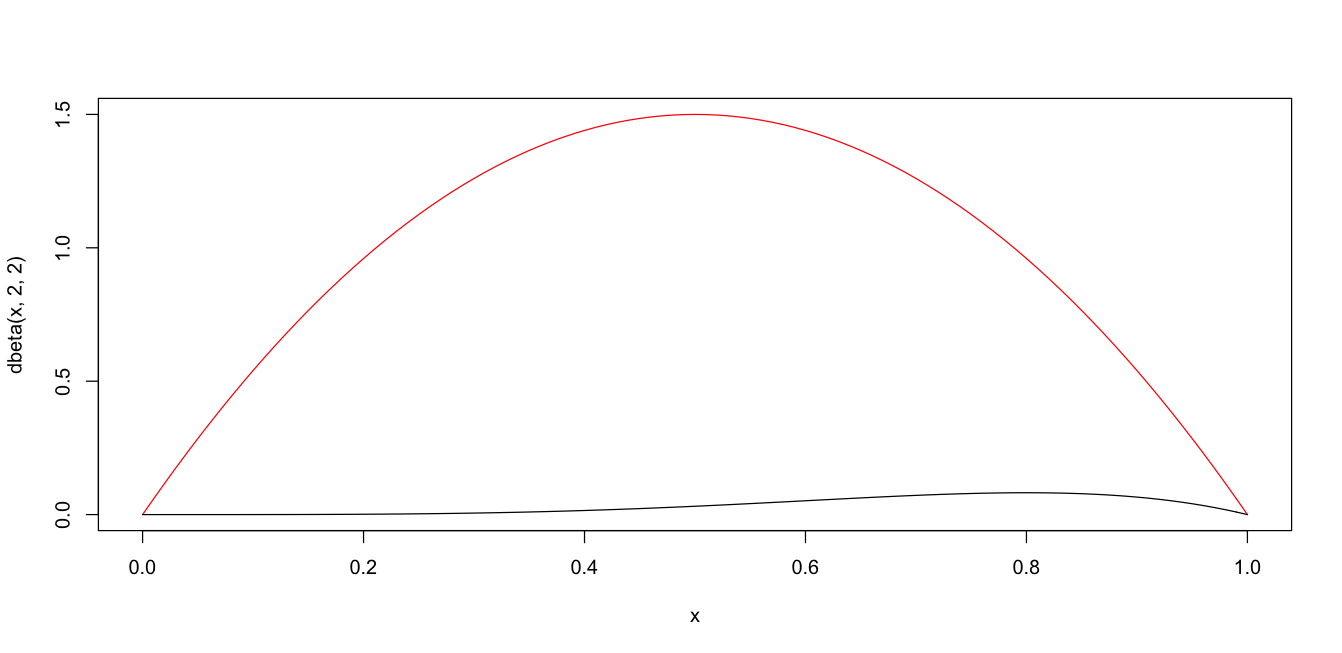
So far so good, but when I try to add the Likelihood function:

likelihood = function(theta) theta^N_1 * (1 - theta)^N_0
curve(likelihood,
      add = T)

with likelihood

They are definitely on different scales. But what multiplication constant am I missing here? Thanks.

$\endgroup$

2 Answers 2

4
$\begingroup$

First of all, in this case, you have the likelihood function of a discrete random variable, so it shows probabilities between zero and one, and the prior is here a continuous random variable with a probability density function that doesn't have an upper bound. Probability density function shows "probability per foot" and it depends on the units of the variable. Even if you had two probability density functions, their units would not be the same, but here there is no reason to expect them to have the same units.

Second, as you noticed, you are not using a normalizing constant for the likelihood, so it doesn't integrate to unity and can take any units. Normalizing constants are not needed for optimization or sampling. You would need them for applying the Bayes theorem directly.

For plotting, you can always re-scale one of the functions by multiplying it by some constant, so they have comparable height on the plot.

$\endgroup$
4
  • 1
    $\begingroup$ Thanks! Yes, I know that normalisation is not needed for sampling, was just wondering in this particular analytical case. I've realised that if I divide the likelihood function by $\Gamma(N_1 + 1, N_0+1)$ it scales it appropriately. I guess it simply transforms the likelihood into a Beta distribution? $\endgroup$
    – Zlo
    Commented Jul 5, 2021 at 15:33
  • 1
    $\begingroup$ The first reason is misleading: densities do have units of measurement and, when these likelihoods are properly normalized, the densities can legitimately be compared. Only the second reason (lack of a normalizing constant) is a valid explanation. $\endgroup$
    – whuber
    Commented Jul 6, 2021 at 11:41
  • 1
    $\begingroup$ @whuber not sure what you are trying to say. They wouldn't have comparable height on the plot, even if properly normalized. Sure, the difference won't be that extreme, but they won't be the same. Depends on what you mean by "comparing" them and the point of the visualization. $\endgroup$
    – Tim
    Commented Jul 6, 2021 at 13:11
  • 1
    $\begingroup$ @Tim On the contrary, they would have comparable heights. Otherwise, normalization can't even make sense: since both plots have identical areas in identical units and span identical horizontal axes in identical units, their heights are comparable, too, and are in identical units. $\endgroup$
    – whuber
    Commented Jul 6, 2021 at 13:36
4
$\begingroup$

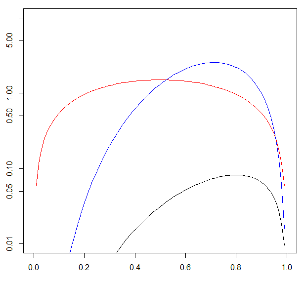
You could try a log scale for the $y$-axis, so the following shows

  • your prior distribution in red
  • your likelihood in black
  • your posterior distribution in blue

You can see the peak of the posterior distribution is further left than the maximum likelihood position

curve(dbeta(x, 2, 2), log="y", ylim=c(0.001,5), col = 'red')
N_1 = 4
N_0 = 1
curve(x^N_1*(1-x)^N_0, add = TRUE, col="black")
curve(dbeta(x, 2+N_1, 2+N_0), add = TRUE, col="blue")

enter image description here

$\endgroup$

Your Answer

By clicking “Post Your Answer”, you agree to our terms of service and acknowledge you have read our privacy policy.

Not the answer you're looking for? Browse other questions tagged or ask your own question.