43
$\begingroup$

I am modeling a random variable ($Y$) which is the sum of some ~15-40k independent Bernoulli random variables ($X_i$), each with a different success probability ($p_i$). Formally, $Y=\sum X_i$ where $\Pr(X_i=1)=p_i$ and $\Pr(X_i=0)=1-p_i$.

I am interested in quickly answering queries such as $\Pr(Y\leq k)$ (where $k$ is given).

Currently, I use random simulations to answer such queries. I randomly draw each $X_i$ according to its $p_i$, then sum all $X_i$ values to get $Y'$. I repeat this process a few thousand times and return the fraction of times $\Pr(Y'\leq k)$.

Obviously, this is not totally accurate (although accuracy greatly increases as the number of simulations increases). Also, it seems I have enough data about the distribution to avoid the use simulations. Can you think of a reasonable way to get the exact probability $\Pr(Y\leq k)$?

p.s.

I use Perl & R.

EDIT

Following the responses I thought some clarifications might be needed. I will shortly describe the setting of my problem. Given is a circular genome with circumference c and a set of n ranges mapped to it. For example, c=3*10^9 and ranges={[100,200],[50,1000],[3*10^9-1,1000],...}. Note all ranges are closed (both ends are inclusive). Also note that we only deal with integers (whole units).

I am looking for regions on the circle that are undercovered by the given n mapped ranges. So to test whether a given a range of length x on the circle is undercovered, I test the hypothesis that the n ranges are mapped randomly. The probability a mapped range of length q>x will fully cover the given range of length x is (q-x)/c. This probability becomes quite small when c is large and/or q is small. What I'm interested is the number of ranges (out of n) which cover x. This is how Y is formed.

I test my null hypothesis vs. one sided alternative (undercoverage). Also note I am testing multiple hypothesis (different x lengths), and sure to correct for this.

$\endgroup$
7
  • $\begingroup$ Are your p_i fixed throughout the modeling exercise or can they change from one calculation to the next? $\endgroup$
    – whuber
    Commented Dec 10, 2010 at 16:30
  • 1
    $\begingroup$ The p_is are fixed. $\endgroup$
    – David B
    Commented Dec 11, 2010 at 13:18
  • $\begingroup$ In light of the current responses, could you share estimates of (a) the sum of the p's and (b) the sum of their squares? These values determine your options. $\endgroup$
    – whuber
    Commented Dec 11, 2010 at 23:53
  • $\begingroup$ @whuber: these greatly vary between cases. It's not a one-time module I'm creating (unfortunately). $\endgroup$
    – David B
    Commented Dec 14, 2010 at 7:09
  • 1
    $\begingroup$ Please consider using sinib package. journal.r-project.org/archive/2018/RJ-2018-011/RJ-2018-011.pdf $\endgroup$
    – Viktor
    Commented Nov 10, 2018 at 3:54

9 Answers 9

27
$\begingroup$

If it often resembles a Poisson, have you tried approximating it by a Poisson with parameter $\lambda = \sum p_i$ ?

EDIT: I've found a theoretical result to justify this, as well as a name for the distribution of $Y$: it's called the Poisson binomial distribution. Le Cam's inequality tells you how closely its distribution is approximated by the distribution of a Poisson with parameter $\lambda = \sum p_i$. It tells you the quality of this approx is governed by the sum of the squares of the $p_i$s, to paraphrase Steele (1994). So if all your $p_i$s are reasonably small, as it now appears they are, it should be a pretty good approximation.

EDIT 2: How small is 'reasonably small'? Well, that depends how good you need the approximation to be! The Wikipedia article on Le Cam's theorem gives the precise form of the result I referred to above: the sum of the absolute differences between the probability mass function (pmf) of $Y$ and the pmf of the above Poisson distribution is no more than twice the sum of the squares of the $p_i$s. Another result from Le Cam (1960) may be easier to use: this sum is also no more than 18 times the largest $p_i$. There are quite a few more such results... see Serfling (1978) for one review.

$\endgroup$
13
  • 1
    $\begingroup$ +1 Not a bad idea. It's likely that a small mixture of Poissons would do a good job, depending on how the question is clarified. $\endgroup$
    – whuber
    Commented Dec 10, 2010 at 18:55
  • 1
    $\begingroup$ I did think about suggesting a negative binomial distribution, which arises as a Gamma-Poisson mixture, but that has a variance larger than its mean, while this problem has a variance smaller than its mean. Based on that, i'm not sure if any mixture of Poissons will work, as surely any such mixture will have variance larger than its mean?? $\endgroup$
    – onestop
    Commented Dec 10, 2010 at 19:25
  • $\begingroup$ @onestop Where was it said that the variance is less than the mean? I missed that statement. $\endgroup$
    – whuber
    Commented Dec 11, 2010 at 7:02
  • $\begingroup$ Sorry whuber, that was a bit cryptic but these comments don't allow that much elaboration. mpiktas's $B_n = \sum p_i(1-p_i)$ is the variance, which is less than the mean, $\sum p_i$. Only slightly less if the $p_i$'s are on average very small though, so standard Poisson might be a good enough approx. Maybe I should expand my answer above.. but then the conversational thread gets confusing. $\endgroup$
    – onestop
    Commented Dec 11, 2010 at 10:40
  • $\begingroup$ What do you mean by $\sum X_i$? How do I get $X_i$ values? $\endgroup$
    – David B
    Commented Dec 11, 2010 at 13:24
12
$\begingroup$

I came across your question while searching for a solution to this very problem. I wasn't terrifically satisfied with the answers here, but I think there's a pretty simple solution that gives you the exact distribution, and is pretty tractable.

The distribution of the sum of two discrete random variables is the convolution of their densities. So if you have $Z = X + Y$ where you know $P(X)$ and $P(Y)$ then you can compute:

$$P(Z=z) = \sum_{k=-\infty}^{\infty} P(X=k) \; P(Y=z-k)$$

(Of course for Bernoulli random variables you don't need to go quite to infinity.)

You can use this to find the exact distribution of the sum of your RVs. First sum two of the RVs together by convolving their PDFs (e.g. [0.3, 0.7] * [0.6, 0.4] = [0.18, 0.54, 0.28]). Then convolve that new distribution with your next Bernoulli PDF (e.g. [0.18, 0.54, 0.28] * [0.5, 0.5] = [0.09, 0.36, 0.41, 0.14]). Keep repeating this until all RVs have been added. And voila, the resulting vector is the exact PDF of the sum of all your variables.

I've verified with simulation that this produces the correct results. It doesn't rely on any asymptotic assumptions, and has no requirements that the Bernoulli probs are small.

There may also be some way to do this more efficiently than repeated convolution, but I haven't thought about it very deeply. I hope this is helpful to somebody!

$\endgroup$
3
  • 2
    $\begingroup$ Have you tried this with 40K variables?? (I wonder how many hours or days of computation it takes...) $\endgroup$
    – whuber
    Commented Mar 23, 2012 at 19:17
  • 6
    $\begingroup$ (+1) I found a way to make this idea work. It requires two techniques: first, use FFT for the convolutions; second, don't do them sequentially, but divide and conquer: do them in disjoint pairs, then do the results in disjoint pairs, etc. The algorithm now scales as $O(n\log n)$ rather than $O(n^2)$ for $n$ probabilities. For instance, Mathematica can compute the entire distribution for 40,000 probabilities in just 0.4 seconds. (1,000,000 are calculated in 10.5 seconds.) I will provide code in a followup comment. $\endgroup$
    – whuber
    Commented Mar 24, 2012 at 18:05
  • 8
    $\begingroup$ Here's the Mathematica code: multinomial[p_] := Module[{lc, condense}, lc = Function[{s}, ListConvolve[s[[1]], s[[2]], {1, -1}, 0]]; condense = Function[{s}, Map[lc, Partition[s, 2, 2, {1, 1}, {{1}}]]]; Flatten[NestWhile[condense, Transpose[{1 - p, p}], Length[#] > 1 &]]] To apply it, do something like p = RandomReal[{0, 1}, 40000]; pp = multinomial[p];. This creates the probabilities p and then computes the exact distribution pp. NB When the mean of p is not extreme, the distribution is very close to normal: that leads to a much faster algorithm yet. $\endgroup$
    – whuber
    Commented Mar 24, 2012 at 18:08
11
$\begingroup$

(Because this is approach is independent of the other solutions posted, including one that I have posted, I'm offering it as a separate response).

You can compute the exact distribution in seconds (or less) provided the sum of the p's is small.

We have already seen suggestions that the distribution might approximately be Gaussian (under some scenarios) or Poisson (under other scenarios). Either way, we know its mean $\mu$ is the sum of the $p_i$ and its variance $\sigma^2$ is the sum of $p_i(1-p_i)$. Therefore the distribution will be concentrated within a few standard deviations of its mean, say $z$ SDs with $z$ between 4 and 6 or thereabouts. Therefore we need only compute the probability that the sum $X$ equals (an integer) $k$ for $k = \mu - z \sigma$ through $k = \mu + z \sigma$. When most of the $p_i$ are small, $\sigma^2$ is approximately equal to (but slightly less than) $\mu$, so to be conservative we can do the computation for $k$ in the interval $[\mu - z \sqrt{\mu}, \mu + z \sqrt{\mu}]$. For example, when the sum of the $p_i$ equals $9$ and choosing $z = 6$ in order to cover the tails well, we would need the computation to cover $k$ in $[9 - 6 \sqrt{9}, 9 + 6 \sqrt{9}]$ = $[0, 27]$, which is just 28 values.

The distribution is computed recursively. Let $f_i$ be the distribution of the sum of the first $i$ of these Bernoulli variables. For any $j$ from $0$ through $i+1$, the sum of the first $i+1$ variables can equal $j$ in two mutually exclusive ways: the sum of the first $i$ variables equals $j$ and the $i+1^\text{st}$ is $0$ or else the sum of the first $i$ variables equals $j-1$ and the $i+1^\text{st}$ is $1$. Therefore

$$f_{i+1}(j) = f_i(j)(1 - p_{i+1}) + f_i(j-1) p_{i+1}.$$

We only need to carry out this computation for integral $j$ in the interval from $\max(0, \mu - z \sqrt{\mu})$ to $\mu + z \sqrt{\mu}.$

When most of the $p_i$ are tiny (but the $1 - p_i$ are still distinguishable from $1$ with reasonable precision), this approach is not plagued with the huge accumulation of floating point roundoff errors used in the solution I previously posted. Therefore, extended-precision computation is not required. For example, a double-precision calculation for an array of $2^{16}$ probabilities $p_i = 1/(i+1)$ ($\mu = 10.6676$, requiring calculations for probabilities of sums between $0$ and $31$) took 0.1 seconds with Mathematica 8 and 1-2 seconds with Excel 2002 (both obtained the same answers). Repeating it with quadruple precision (in Mathematica) took about 2 seconds but did not change any answer by more than $3 \times 10^{-15}$. Terminating the distribution at $z = 6$ SDs into the upper tail lost only $3.6 \times 10^{-8}$ of the total probability.

Another calculation for an array of 40,000 double precision random values between 0 and 0.001 ($\mu = 19.9093$) took 0.08 seconds with Mathematica.

This algorithm is parallelizable. Just break the set of $p_i$ into disjoint subsets of approximately equal size, one per processor. Compute the distribution for each subset, then convolve the results (using FFT if you like, although this speedup is probably unnecessary) to obtain the full answer. This makes it practical to use even when $\mu$ gets large, when you need to look far out into the tails ($z$ large), and/or $n$ is large.

The timing for an array of $n$ variables with $m$ processors scales as $O(n(\mu + z \sqrt{\mu})/m)$. Mathematica's speed is on the order of a million per second. For example, with $m = 1$ processor, $n = 20000$ variates, a total probability of $\mu = 100$, and going out to $z = 6$ standard deviations into the upper tail, $n(\mu + z \sqrt{\mu})/m = 3.2$ million: figure a couple seconds of computing time. If you compile this you might speed up the performance two orders of magnitude.

Incidentally, in these test cases, graphs of the distribution clearly showed some positive skewness: they aren't normal.

For the record, here is a Mathematica solution:

pb[p_, z_] := Module[
  {\[Mu] = Total[p]},
  Fold[#1 - #2 Differences[Prepend[#1, 0]] &, 
   Prepend[ConstantArray[0, Ceiling[\[Mu] + Sqrt[\[Mu]] z]], 1], p]
  ]

(NB The color coding applied by this site is meaningless for Mathematica code. In particular, the gray stuff is not comments: it's where all the work is done!)

An example of its use is

pb[RandomReal[{0, 0.001}, 40000], 8]

Edit

An R solution is ten times slower than Mathematica in this test case--perhaps I have not coded it optimally--but it still executes quickly (about one second):

pb <- function(p, z) {
  mu <- sum(p)
  x <- c(1, rep(0, ceiling(mu + sqrt(mu) * z)))
  f <- function(v) {x <<- x - v * diff(c(0, x));}
  sapply(p, f); x  
}
y <- pb(runif(40000, 0, 0.001), 8)
plot(y)
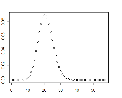
Plot of PDF

$\endgroup$
0
9
$\begingroup$

@onestop provides good references. The Wikipedia article on the Poisson binomial distribution gives a recursive formula for computing the exact probability distribution; it requires $O(n^2)$ effort. Unfortunately, it's an alternating sum, so it will be numerically unstable: it's hopeless to do this computation with floating point arithmetic. Fortunately, when the $p_i$ are small, you only need to compute a small number of probabilities, so the effort is really proportional to $O(n \log(\sum_i{p_i}))$. The precision necessary to carry out the calculation with rational arithmetic (i.e., exactly, so that the numerical instability is not a problem) grows slowly enough that the overall timing may still be approximately $O(n^2)$. That's feasible.

As a test, I created an array of probabilities $p_i = 1/(i+1)$ for various values of $n$ up to $n = 2^{16}$, which is the size of this problem. For small values of $n$ (up to $n = 2^{12}$) the timing for the exact calculation of probabilities was in seconds and scaled quadratically, so I ventured a calculation for $n = 2^{16}$ out to three SDs above the mean (probabilities for 0, 1, ..., 22 successes). It took 80 minutes (with Mathematica 8), in line with the predicted time. (The resulting probabilities are fractions whose numerators and denominators have about 75,000 digits apiece!) This shows the calculation can be done.

An alternative is to run a long simulation (a million trials ought to do). It only has to be done once, because the $p_i$ don't change.

$\endgroup$
0
8
$\begingroup$

With different $p_i$ your best bet I think is normal approximation. Let $B_n=\sum_{i=1}^np_i(1-p_i)$. Then

\begin{align*} B_n^{-1/2}\left(\sum_{i=1}^nX_i-\sum_{i=1}^np_i\right)\to N(0,1), \end{align*} as $n\to\infty$, provided that for each $\varepsilon>0$

\begin{align*} B_n^{-1}\sum_{i=1}^nE\left((X_i-p_i)^2\mathbf{1}\{|X_i-p_i|>\varepsilon B_n^{1/2}\}\right)\to 0, \end{align*} as $n\to\infty$, which for Bernoulli variables will hold if $B_n\to\infty$. This is the so-called Lindeberg condition, which is sufficient and necessary for convergence to the standard normal.

Update: The approximation error can be calculated from the following inequality:

\begin{align*} \sup_x|F_n(x)-\Phi(x)|\le AL_n, \end{align*} where \begin{align*} L_n=B_n^{-3/2}\sum_{i=1}^nE|X_i-p_i|^3 \end{align*} and $F_n$ is the cdf of the scaled and centered sum of $X_i$.

As whuber pointed out, the convergence can be slow for badly behaved $p_i$. For $p_i=\frac{1}{1+i}$ we have $B_n\approx \ln n$ and $L_n\approx (\ln n)^{-1/2}$. Then taking $n=2^{16}$ we get that the maximum deviation from the standard normal cdf is a whopping 0.3.

$\endgroup$
9
  • 3
    $\begingroup$ This is not true when the p_i approach zero as i increases. Otherwise, you have just proven that the Poisson distribution is Normal! $\endgroup$
    – whuber
    Commented Dec 10, 2010 at 16:14
  • 1
    $\begingroup$ That is why it must be $B_n\to\infty$. If $p_i$ approach zero at rate faster than $1/i$, $\lim B_n<\infty$. $\endgroup$
    – mpiktas
    Commented Dec 10, 2010 at 17:58
  • $\begingroup$ @mpiktas is right. The analogy to the Poisson distribution doesn't quite fit, here. $\endgroup$
    – user1108
    Commented Dec 10, 2010 at 18:12
  • $\begingroup$ By the way, I didn't actually check that monstrous condition in the second paragraph. $\endgroup$
    – user1108
    Commented Dec 10, 2010 at 18:22
  • $\begingroup$ @G. Jay Kerns I agree that the analogy to the Poisson is imperfect, but I think it gives good guidance. Imagine a sequence of p's, p_i = 10^{-j}, where j is the order of magnitude of i (equal to 1 for i <= 10, to 2 for i <= 100, etc.). When n = 10^k, 90% of the p's equal 10^{-k} and their sum looks Poisson with expectation 0.9. Another 9% equal 10^{1-k} and their sum looks Poisson (with the same expectation). Thus the distribution looks approximately like a sum of k Poisson variates. It's obviously nowhere near Normal. Whence the need for the "monstrous condition." $\endgroup$
    – whuber
    Commented Dec 10, 2010 at 18:53
4
$\begingroup$

Well, based on your description and the discussion in the comments it is clear that $Y$ has mean $\sum_i p_i$ and variance $\sum_i p_{i}(1-p_{i})$. The shape of $Y$'s distribution will ultimately depend on the behavior of $p_i$. For suitably "nice" $p_i$ (in the sense that not too many of them are really close to zero), the distribution of $Y$ will be approximately normal (centered right at $\sum p_i$). But as $\sum_i p_i$ starts heading toward zero the distribution will be shifted to the left and when it crowds up against the $y$-axis it will start looking a lot less normal and a lot more Poisson, as @whuber and @onestop have mentioned.

From your comment "the distribution looks Poisson" I suspect that this latter case is what's happening, but can't really be sure without some sort of visual display or summary statistics about the $p$'s. Note however, as @whuber did, that with sufficiently pathological behavior of the $p$'s you can have all sorts of spooky things happen, like limits that are mixture distributions. I doubt that is the case here, but again, it really depends on what your $p$'s are doing.

As to the original question of "how to efficiently model", I was going to suggest a hierarchical model for you but it isn't really appropriate if the $p$'s are fixed constants. In short, take a look at a histogram of the $p$'s and make a first guess based on what you see. I would recommend the answer by @mpiktas (and by extension @csgillespie) if your $p$'s aren't too crowded to the left, and I would recommend the answer by @onestop if they are crowded left-ly.

By the way, here is the R code I used while playing around with this problem: the code isn't really appropriate if your $p$'s are too small, but it should be easy to plug in different models for $p$ (including spooky-crazy ones) to see what happens to the ultimate distribution of $Y$.

set.seed(1)
M <- 5000
N <- 15000
p <- rbeta(N, shape1 = 1, shape2 = 10)
Y <- replicate(M, sum(rbinom(N, size = 1, prob = p)))

Now take a look at the results.

hist(Y)
mean(Y)
sum(p)
var(Y)
sum(p*(1 - p))

Have fun; I sure did.

$\endgroup$
2
  • $\begingroup$ Why do you say "the code isn't really appropriate if your $p$s are too small"? Seems to work ok to me, e.g. with shape1=1, shape2=999, giving a mean $p$ of 0.001. $\endgroup$
    – onestop
    Commented Dec 11, 2010 at 22:07
  • $\begingroup$ @onestop what I meant was the specific choice of (1,10) written above doesn't give values of $p$ that are very small, to the point that the normal approximation looks pretty good. If a person wanted the Poisson to come out then they would need to try something else; it sounds like your choice of (1,999) does a good job, yes? I had also thought to make $\alpha < 1$, say, 0.25, but I haven't tried that. $\endgroup$
    – user1108
    Commented Dec 12, 2010 at 2:55
3
$\begingroup$

I think other answers are great, but I didn't see any Bayesian ways of estimating your probability. The answer doesn't have an explicit form, but the probability can be simulated using R.

Here is the attempt:

$$ X_i | p_i \sim Ber(p_i)$$

$$ p_i \sim Beta(\alpha, \beta) $$

Using wikipedia we can get estimates of $\hat{\alpha}$ and $\hat{\beta}$ (see parameter estimation section).

Now you can generate draws for the $i^{th}$ step, generate $p_i$ from $Beta(\hat{\alpha},\hat{\beta})$ and then generate $ X_i$ from $Ber(p_i)$. After you have done this $N$ times you can get $Y = \sum X_i$. This is a single cycle for generation of Y, do this $M$(large) number of times and the histogram for $M$ Ys will be the estimate of density of Y.

$$Prob[Y \leq y] = \frac {\#Y \leq y} {M}$$

This analysis is valid only when $p_i$ are not fixed. This is not the case here. But I will leave it here, in case someone has a similar question.

$\endgroup$
4
  • 2
    $\begingroup$ To some purists this may not be Bayesian. This is actually empirical Bayesian, but it is a quick way to simulate your probabilities in R, without resorting to hyper prior mumbo jumbo. $\endgroup$
    – suncoolsu
    Commented Dec 12, 2010 at 3:41
  • 1
    $\begingroup$ Why do you need priors when the p_i are given? $\endgroup$
    – whuber
    Commented Dec 12, 2010 at 22:55
  • $\begingroup$ @whuber. Thanks, you are right. I missed the fixed part. I thought David is just using the value to be $p_i$ as (q-x)/c and is not fixed. I will edit my answer. $\endgroup$
    – suncoolsu
    Commented Dec 12, 2010 at 23:58
  • 1
    $\begingroup$ @suncoolsu - note that a "beta-bernoulli" distribution is just another bernoulli distribution but replacing $p_i\to\frac{\alpha}{\alpha+\beta}$. This is becase ${1\choose x_i}\frac{B(\alpha+x_i,\beta+1-x_i)}{B(\alpha,\beta)}=\frac{\alpha^{x_i}\beta^{1-x_i}}{\alpha+\beta}$. So basically by mixing over $p_i$ you are applying the binomial approximation here $p_1=p_2=\dots=p_n$. $\endgroup$ Commented Dec 3, 2013 at 14:08
3
$\begingroup$

I would suggest applying Poisson approximation. It is well known (see A. D. Barbour, L. Holst and S. Janson: Poisson Approximation) that the total variation distance between $Y$ and a r.v. $Z$ having Poisson distribution with the parameter $\sum_i p_i$ is small: $$ \sup_A |{\bf P}(Y\in A) - {\bf P}(Z\in A)| \le \min \left\{ 1, \frac{1}{\sum_i p_i} \right\} \sum_i p_i^2. $$ There are also bounds in terms of information divergence (the Kullback-Leibler distance, you may see P. Harremoёs: Convergence to the Poisson Distribution in Information Divergence. Preprint no. 2, Feb. 2003, Mathematical Department, University of Copenhagen. http://www.harremoes.dk/Peter/poisprep.pdf and other publications of P.Harremoёs), chi-squared distance (see Borisov and Vorozheikin https://link.springer.com/article/10.1007%2Fs11202-008-0002-3) and some other distances.

For the accuracy of approximation $|{\bf E}f(Y) - {\bf E}f(Z)|$ for unbounded functions $f$ you may see Borisov and Ruzankin https://projecteuclid.org/euclid.aop/1039548369 . Besides, that paper contains a simple bound for probabilities: for all $A$, we have $${\bf P}(Y\in A) \le \frac{1}{(1-\max_i p_i)^2} {\bf P}(Z\in A).$$

$\endgroup$
1
  • 2
    $\begingroup$ +1 Thank you for the useful quantitative information about the approximation bounds. Welcome to our site! $\endgroup$
    – whuber
    Commented Nov 10, 2018 at 13:22
2
$\begingroup$

As has been mentioned in other answers, the probability distribution you describe is the Poisson Binomial distribution. An efficient method for computing the CDF is given in Hong, Yili. On computing the distribution function for the Poisson binomial distribution.

The approach is to efficiently compute the DFT (discrete Fourier transform) of the characteristic function.

The characteristic function of the Poisson binomial distribution is give by $\phi(t) = \prod_j^n [(1-p_j)+p_je^{it}]$ ($i=\sqrt{-1}$).

The algorithm is:

  1. Let $z_j(k) = 1-p_j+p_j \text{cos}(\omega k)+ i p_j \text{sin}(\omega k)$, for $\omega=\frac{2\pi}{n+1}$.
  2. Define $x_k=\text{exp}\{\sum_j^n log(z_j(k))\}$, define $x_0=1$.
  3. Compute $x_k$ for $k=1,\dots,[n/2]$. Use symmetry $\bar{x}_k=x_{n+1-k}$ to get the rest.
  4. Apply FFT to the vector $\frac{1}{n+1}<x_0,x_1,\dots,x_n>$.
  5. Take the cumulative sum of result to get the CDF.

The algorithm is available in the poibin R package.

This approach gives much better results than the recursive formulations as they tend to lack numerical stability.

$\endgroup$
1
  • 5
    $\begingroup$ I have access only to the abstract of that paper, but it sounds like it implements the method I used at stats.stackexchange.com/questions/41247/… and discusses how it performs compares to the other methods given in this thread. If you know more about what the paper has accomplished, we would be glad to read a summary. $\endgroup$
    – whuber
    Commented Nov 2, 2017 at 19:04

Your Answer

By clicking “Post Your Answer”, you agree to our terms of service and acknowledge you have read our privacy policy.

Not the answer you're looking for? Browse other questions tagged or ask your own question.