The simplest technique in your case is to calculate the correlation $r$ of de-meaned signals, then get the phase difference as $\phi=\arccos(r/\pi)$ if the signals are harmonic, i.e. single frequency sine waves.
Another way of doing this is with cross-correlation function. The idea is to calculate the correlation between one signal and the lagged second signal. When the number of lags is closest to the phase shift, you'll get the maximum correlation. The advantage of this technique is that it doesn't depend on the shape of your signal, while the first method is best for harmonic signals.
correlation method
Why should this work for you? At the sampling frequency of 500MHz, you have at least 36 points of each wave of your 13.56MHz signal. With 20000 samples gives you hundreds of full waves measured, which means that the average of signals will be very close to the means and the partial waves at the beginning and end of your samples will not be important. Thus, after de-meaning the signals, the correlation simply boils down to the following equation:
$$r\approx\frac{\int_0^{2\pi}sin(x)sin(x+\phi)}{\int_0^{2\pi}sin(x)^2}=\cos(\phi)$$
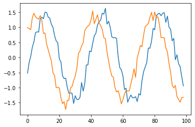
Here's a piece of Python code to demonstrate how this works for noise/signal ratio 10%.
import numpy as np
import math

# create fake data
nsr = 1e-1
r = np.random.normal(size=(20000,2)) * nsr
phdiff = math.pi * np.random.uniform()
print('true phase diff (radians):', phdiff, '\t(degrees):', phdiff / (2 * math.pi) * 360)
omega = 13.56e6
t = np.arange(20000) / 500e6
rdata = np.zeros((len(t), 2))
ph0 = 2 * math.pi * np.random.uniform()
rdata[:,0] = np.sin(2 * math.pi * omega * t + ph0)
rdata[:,1] = np.sin(2 * math.pi * omega * t + phdiff + ph0)
rdata = rdata + r

# scale
from sklearn.preprocessing import StandardScaler
scaler = StandardScaler()
scaler.fit(rdata)
data = scaler.transform(rdata)

import matplotlib.pyplot as plt
plt.figure()
plt.plot(data[1:100,:])
plt.show()

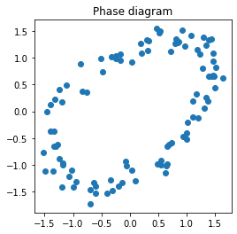
# phase difference determination
plt.figure(figsize=(4,4))
plt.title('Phase diagram')
plt.scatter(data[1:100,0],data[1:100,1])
plt.show()

c = np.cov(np.transpose(data))
print('cov: ', c)
phi = np.arccos(c[0,1] )
print('phase estimate (radians): ', phi, '(degrees): ', phi / math.pi * 180)
Output:
true phase diff (radians): 1.049746982742775    (degrees): 60.146071667753475

cov:  [[1.00005    0.48973754]
 [0.48973754 1.00005   ]]
phase estimate (radians):  1.059007630672643 (degrees):  60.67666770969148


cross-correlation method
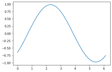
Here's a piece of code to demonstrate how it could work.
from statsmodels.tsa.stattools import ccf
xc = ccf(data[:,0], data[:,1])
plt.figure()
angle = t * omega * 2 * math.pi

n = math.ceil(fs / omega)
plt.plot(angle[:n], xc[:n])
plt.show()
print(angle)

maxa = max(np.abs(xc[:int(n/2)]))
maxangle = angle[np.abs(xc)==maxa]
print('phase shift (radians): ',maxangle)
Output:

phase shift (radians): [2.3855998]
PCA
My initial answer with PCA, but it's more complicated. You can run PCA on the standardized signals, then the ratio of explained variances will contain information about the phase difference of the signals.

