2
$\begingroup$

I have a set of data that represent the sum of white matter streamlines termination in 64 regions of interest in the brain surface collected from 40 subjects. Below is an example of a paired data of one region for both right and left brain hemispheres. The variable "value" represents the sum of all streamlines that terminated within this region.

side <- c("Right","Right","Right","Right","Right","Right","Right","Right","Right","Right","Right","Right","Right","Right","Right","Right","Right","Right","Right","Right","Right","Right","Right","Right","Right","Right","Right","Right","Right","Right","Right","Right","Right","Right","Right","Right","Right","Right","Right","Right","Left","Left","Left","Left","Left","Left","Left","Left","Left","Left","Left","Left","Left","Left","Left","Left","Left","Left","Left","Left","Left","Left","Left","Left","Left","Left","Left","Left","Left","Left","Left","Left","Left","Left","Left","Left","Left","Left","Left","Left")

value <- c(0,0,0,306,4,156,2,3,0,146,0,218,0,0,74,5,0,833,0,640,76,49,0,0,163,65,0,0,5,14,2,0,92,229,0,23,338,0,0,11,90,51,0,4,394,50,138,0,12,481,325,237,0,574,102,391,2,104,559,0,348,427,554,214,786,312,407,45,356,114,19,104,194,833,192,354,126,4,716,129)

data <- data.frame(side, value)

head(data)

   side value
1 Right     0
2 Right     0
3 Right     0
4 Right   306
5 Right     4
6 Right   156

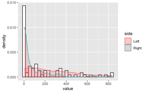
As can be seen, several subjects ended with zero value, especially on the right side. When looking into the distribution of the data as below, the right side data is highly skewed due to zero inflation.

ggplot(data, aes(x = value, color = side)) + 
  geom_histogram(aes(y=..density..), colour="black", fill="white") + 
                   geom_density(alpha=.2, fill="#FF6666")

enter image description here

These zero values are true zeros and have to be included in my analysis. It is normal for the brain areas to have zero values of certain white matter streamlines.

My purpose is to test the mean difference and to bring a parameter estimate or an effect size measurement to plot for visualization. My null hypothesis is that there is no significant difference between the two sides. Can the Wilcoxon signed-rank test still be used with such data? I am using R but can use SPSS if required.

$\endgroup$
2
  • $\begingroup$ However, I am concerned that neither your data nor your display indicate which values are paired with which; it should be explicit (and I fear that as presently organized, it would be too easy to end up scrambling the order and lose however the pairing is currently set up). $\endgroup$
    – Glen_b
    Commented Sep 5, 2021 at 4:19
  • $\begingroup$ Thanks Glen for the comments. Can you elaborate more about the alternative you mentioned. Regarding the pairing of the data, no worries even with the split done by Jan I can confirm it is accurately paired. $\endgroup$ Commented Sep 5, 2021 at 5:16

2 Answers 2

1
$\begingroup$

Yes a paired wilcoxon test is inappropriate in this case. Since you want to test the mean but your data is highly skewed and I checked that 25 per cent of the values are outliers you could use a dependent Yuen's t-test on 25 per cent trimmed means. In R you can do this easily with the yuend function from the package WRS2:

# convert data to wide list format:

> data <- split(value, list(side))

library(WRS2)

> yuend(data$Left, data$Right, tr = 0.25)
Call:
yuend(x = data$Left, y = data$Right, tr = 0.25)

Test statistic: 3.804 (df = 19), p-value = 0.0012

Trimmed mean difference:  179.9 
95 percent confidence interval:
80.9156     278.8844 

Explanatory measure of effect size: 0.69 

# 25% trimmed mean group 'Left':

> mean(data$Left, tr = 0.25)
[1] 196.55


# 25% trimmed mean group 'Right':
> mean(data$Right, tr = 0.25)
[1] 16.65

So you see that we measure significantly lower values in the right group. Moreover, the effect size $\xi$ suggests a large effect.

$\endgroup$
4
  • $\begingroup$ Thank you Jan for the quick reply. I had the robust analysis in my mind but since I have no experience with it I was reluctant to use it, but your answer encouraged me to go with it. One more question, I have 40 subjects with 64 regions in each case. Does that mean I shall confirm the percentage of zeros for each region to decide the trim value? $\endgroup$ Commented Sep 4, 2021 at 11:56
  • $\begingroup$ No, generally you select the amount of trimming by looking at the DV's percentage of outliers and/or the standard error for a particular trimming amount (the lower the standard error the more accurately is your measure of location representing your data). In your example the 25% trimmed mean has the lowest standard error. Check by yourself. Use trimse(value, tr = 0.25) and change the tr argument e.g. to 0 or 0.10. $\endgroup$
    – Jan
    Commented Sep 4, 2021 at 12:33
  • $\begingroup$ Thanks again Jan. $\endgroup$ Commented Sep 4, 2021 at 12:55
  • $\begingroup$ You're welcome Mudathir. Glad I could help. $\endgroup$
    – Jan
    Commented Sep 4, 2021 at 16:40
2
$\begingroup$

In relation to the title question I think that it's okay, at least under some conditions. I would be inclined to omit the observations that are the difference of two 0's as contributing no information about the difference rather than simply apply an adjustment of ties. (In any case, certainly we cannot just enter them all as if we were dealing with continuous comparisons.)

However, if you're interested in a mean difference, I would not at first glance suggest a signed rank test since it also does not correspond to the hypothesis about population means without additional assumptions.

There are several potential alternatives for testing means. Here are some:

  1. A plain permutation test of means.

  2. Come up with a suitable parametric model and then derive a good test for comparing means; ideally with some knowledge of the likely behavior of the quantities. (In this case I don't have enough domain knowledge to say much of anything but it seems that the non-zero measurements are on the positive half-line and perhaps a zero-inflated gamma might be adequate.)

  3. Start with the exercise in 2. to arrive at a hopefully plausible model, but rather than rely on it being quite correct, use it as the basis of a permutation test. This may require additional assumptions to make it a suitable test of means if the model is not quite right.

  4. Use a bootstrap test.

  5. After checking that the type I error rate is not going to be too far off with n=40, on distributions that looks something like the one at hand, simply use a paired t-test.

    Even when the significance level is fine, this may result in some loss of power relative to a more suitable model (there's not much tendency for relative efficiency to improve with sample size). This may or may not be a major issue, depending on circumstances.

  6. Make the additional assumptions necessary to use a signed rank test (or indeed any other test, such as a robust test) to compare population means, and adjust the approach to deal with the issue with the differences of two 0s.

$\endgroup$
5
  • $\begingroup$ Thank you for the detailed explanation. For a newbie like me, I will need to study these options intensively to make a decision. However, I am deeply interested in number 5, because I have read a similar opinion before. Can I understand from the discussion made on this topic, that there are no agreed-upon solid guidelines to deal with such data? In other words, (me) as a physician who is asking, are there method's preferences among statisticians, or is it still a matter of argument and discussion? $\endgroup$ Commented Sep 6, 2021 at 3:59
  • $\begingroup$ 1. There are indeed multiple methods in use by statisticians; different ones will choose different options (in your case I'd have probably built a Bayesian model, personally, but on the other hand I may instead have done some work with a zero-inflated GLM). But these don't usually begin with the data you want to run inference on. 2. I tend to choose distributional models with care after (a) considerable effort investigating the nature of the response variables, starting with their support, and considering things like whether we could expect variance to increase when the mean increases,...ctd $\endgroup$
    – Glen_b
    Commented Sep 6, 2021 at 5:12
  • $\begingroup$ ctd... along with looking at any previous data (prior studies, pilot samples, similar variables), talking to experts about that variable and so forth. This is particularly important if sample sizes are going to be low, since parametric models become more important; and (b) considering the particular purposes of the analysis, and where necessary its potential audience. All this is, as absolutely far as possible, done before any sampling (because if you have to do it after by looking at some of your data, you either lose some valuable data or you will muck up the properties of your analyses). $\endgroup$
    – Glen_b
    Commented Sep 6, 2021 at 5:12
  • $\begingroup$ I'll think about whether I can say more of value under point 5. $\endgroup$
    – Glen_b
    Commented Sep 6, 2021 at 5:13
  • $\begingroup$ Thanks again Glen, you have been generous with your knowledge. I understand that it might be ideal from a statistical point of view and I appreciate your time to teach me and I enjoyed it. I am glad you brought up the issue of "potential audience" since they are mostly surgeons and the majority of them have no interest in the details of the analysis. The example I introduced here was one pair out of 2560. It will be challenging since all pairs won't share a certain distribution. I will wait for your comment about point 5. $\endgroup$ Commented Sep 6, 2021 at 9:00

Your Answer

By clicking “Post Your Answer”, you agree to our terms of service and acknowledge you have read our privacy policy.

Not the answer you're looking for? Browse other questions tagged or ask your own question.