Background and theory
In relation to what @Ben said, you could apply the gatekeeping procedure described in Bretz et al. (2009). First, fit the following regression model:
$$
y_i=\beta_0 + \beta_1\,\mathrm{Group}_{2, i} + \beta_2\,\mathrm{Subgroup}_{2, i} + \beta_3\,\mathrm{Group}_{2, i}\times\mathrm{Subgroup}_{2, i}
$$
where $\mathrm{Group}_{2}$ and $\mathrm{Subgroup}_{2}$ are indicator variables for the second group and subgroup, respectively. According to this model, we would have three null hypotheses:
\begin{align}
\operatorname{H}_{1}:&~ \beta_1 = \beta_2 = \beta_3 = 0 \\
\operatorname{H}_{2}:&~ \beta_2 = 0 \\
\operatorname{H}_{3}:&~ \beta_2 + \beta_3 = 0 \\
\end{align}
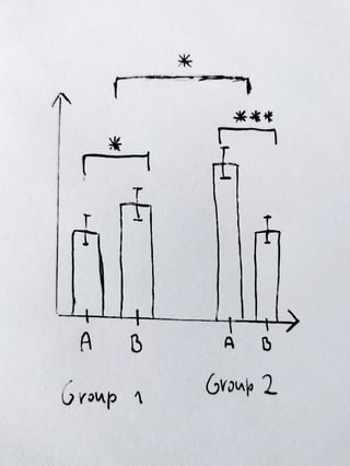
$\operatorname{H}_{1}$ poses that all four means are equal. $\operatorname{H}_{2}$ is your first hypothesis that the means of $A$ and $B$ are equal in Group 1. To see this, consider how the means for subgroup 1 ($A$) and 2 ($B$) in group 1 are parametrized in the model above:
\begin{align}
\mu_{1, A} &= \beta_0 + \beta_1\,0 + \beta_2\,0 + \beta_3\,0\times0 = \beta_0 \\
\mu_{1, B} &= \beta_0 + \beta_1\,0 + \beta_2\,1 + \beta_3\,0\times0 = \beta_0 + \beta_2
\end{align}
So the difference between the two subgroups in group 1 corresponds to $\beta_2$ in the model and testing the null hypothesis that $\beta_2 = 0$ corresponds to testing if there is a difference between subgroups 1 and 2 within group 1.Further, $\operatorname{H}_{3}$ corresponds to your second hypothesis that the means of $A$ and $B$ are equal in Group 2. What's special is that we only consider $\operatorname{H}_{2}$ and $\operatorname{H}_{3}$ when $\operatorname{H}_{1}$ is providing evidence against the null hypothesis (i.e. $\operatorname{H}_{1}$ is rejected). Your third hypothesis can easily be accomodated by the procedure described here.
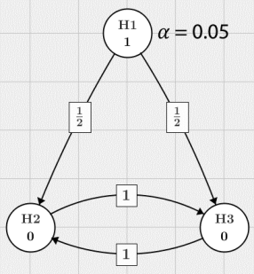
According to Bretz et al. (2009), we can visualize the structure among the hypohteses using the following graph:

There is only one gatekeeping hypothesis so it gets a weight of 1. We also like to control the overall familywise error rate (FWER) at $\alpha = 0.05$. The first hypothesis is connected to the other two via an edge with a weight of $1/2$. This means that if we reject $\operatorname{H}_{1}$ at $\alpha$, this local level is split equally and transferred to $\operatorname{H}_{2}$ and $\operatorname{H}_{3}$ which are then tested at $\alpha/2$ in this case. Furthermore, $\operatorname{H}_{2}$
and $\operatorname{H}_{3}$ are connected via edges with weight 1 which means that if $\operatorname{H}_{2}$ ($\operatorname{H}_{3}$) is rejected at its local level, this
level is passed to $\operatorname{H}_{3}$ ($\operatorname{H}_{2}$).
In this case, this means that if $\operatorname{H}_{1}$ is rejected at $\alpha$, you would use the Bonferroni-Holm procedure for the two remaining hypotheses. For more complex graphs, refer to the algorithm described in Bretz et al. (2009) for calculating the adjusted $p$-values (see below for an R package that does this for you).
Example and implementation
The first hypothesis $\operatorname{H}_{1}$ can be tested using the overall $F$-test of the regression model described above. $\operatorname{H}_{2}$ is a simple $t$-test within the regression model and $\operatorname{H}_{3}$ can also be tested by an $F$-test. Here is an example of the procedure described above using artificial data in R. I assume that the subgroups in group $1$ do not differ while they do within group $2$. This corresponds to assuming $\beta_2 = 0$ in the model above (i.e. $\operatorname{H}_{1}$ and $\operatorname{H}_{3}$ are false and $\operatorname{H}_{2}$ is true):
library(multcomp)

# Sample size per subgroup
n <- 100

# Means and standard deviation for all four subgroups
mu_vec <- c(10, 10, 15, 25)
sigma <- 6

# Generate data
set.seed(142857)

dat <- data.frame(
  y = c(rnorm(n, mu_vec[1], sigma), rnorm(n, mu_vec[2], sigma), rnorm(n, mu_vec[3], sigma), rnorm(n, mu_vec[4], sigma))
  , subg = factor(rep(c("A", "B"), each = n, times = 2))
  , group = factor(rep(1:2, each = 2*n))
)

# Fit regression model
mod <- lm(y~group*subg, data = dat)

# Use glht (multcomp) to calculate the p-values of all hypotheses

H1 <- matrix(c(
  0, 1, 0, 0,
  0, 0, 1, 0,
  0, 0, 0, 1
), ncol = 4, byrow = TRUE)

H1test <- glht(mod, linfct = H1, rhs = 0)
summary(H1test, test = Ftest())

Global Test:
      F DF1 DF2    Pr(>F)
1 166.4   3 396 8.891e-70

H2 <- matrix(c(
  0, 0, 1, 0
), ncol = 4, byrow = TRUE)

H2test <- glht(mod, linfct = H2, rhs = 0)
summary(H2test, test = Ftest())

Global Test:
        F DF1 DF2 Pr(>F)
1 0.01327   1 396 0.9083

H3 <- matrix(c(
  0, 0, 1, 1
), ncol = 4, byrow = TRUE)

H3test <- glht(mod, linfct = H3, rhs = 0)
summary(H3test, test = Ftest())

Global Test:
      F DF1 DF2    Pr(>F)
1 140.7   1 396 5.638e-28
Here, I used glht with contrast matrices for all hypotheses but you could use the regression output for $\operatorname{H}_{1}$ and $\operatorname{H}_{2}$. The $p$-values are extremely small for $\operatorname{H}_{1}$ and $\operatorname{H}_{3}$ and $0.9083$ for $\operatorname{H}_{2}$.
According to the gatekeeping procedure, we reject $\operatorname{H}_{1}$ at the $0.05$ level in the first step. In the second step, we use the Bonferroni-Holm procedure to adjust the $p$-values for $\operatorname{H}_{2}$ and $\operatorname{H}_{3}$, which results in adjusted $p$-values of $0.9083$ and $1.1276\times 10^{-27}$:
p.adjust(c(0.9083, 5.638e-28), "holm")
[1] 9.0830e-01 1.1276e-27
Hence, we reject $\operatorname{H}_{3}$ and fail to reject $\operatorname{H}_{2}$.
This can be automated using the gMCP package for R that implements the algorithms of Bretz et al. (2009). There is a graphical interface but here is the code to do the computations:
library(gMCP)

m <- rbind(H1=c(0, 0.5, 0.5),
           H2=c(0, 0, 1),
           H3=c(0, 1, 0))

weights <- c(1, 0, 0)

graph <- new("graphMCP", m = m, weights = weights)
pvalues <- c(8.891e-70, 0.9083, 5.638e-28)
res <- gMCP(graph, pvalues, test = "Bonferroni", alpha = 0.05)
res

P-values:
       H1        H2        H3
8.891e-70 9.083e-01 5.638e-28

Adjusted p-values:
        H1         H2         H3
8.8910e-70 9.0830e-01 1.1276e-27

Alpha: 0.05

Hypothesis rejected:
   H1    H2    H3
 TRUE FALSE  TRUE
Reference
Bretz, F., Maurer, W., Brannath, W., & Posch, M. (2009). A graphical approach to sequentially rejective multiple test procedures. Statistics in medicine, 28(4), 586-604.


