According to the Wikipedia encyclopedia
In statistics, multicollinearity (also collinearity) is a phenomenon in which one predictor variable in a multiple regression model can be linearly predicted from the others with a substantial degree of accuracy.
So multicollinearity is a special case of correlation. It is more specific in two ways
- It relates specifically to the predictor variables in a regression model.
- It relates to correlation with a linear combination of multiple variables combined.
Correlation doesn't need to be that linear combination of multiple variables (correlation is about two variables). And correlation describes a much wider phenomena than just this case with predictor variables.
There is a distinction between perfect multicollinearity (a perfect linear relation between variables/predictors) or just multicollinearity (not an exact linear relationship but strong correlation of at least one of the predictors with a linear combination of the other predictors).
Is checking for multicollinearity the same as checking for correlation?
No, not exactly.
what is the difference between multicollinearity and correlation? How do I check mathematically multicollinearity? What kind of math is behind this?
Multicollinearity may occur even when there is little correlation present between individual pairs of predictors. The issue of multicollinearity can occur when there is correlation with one predictor and a linear sum of the other predictors.
Imagine for instance when there are six predictors and a seventh is added as the sum $X_7 = X_1 + X_2 + X_ 3 + X_4 + X_5 + X_6$. The correlation between $X_7$ and the other predictors will only be relatively small. But there will be perfect multicollinearity.
In that example of perfect linear relationship, you can check perfect multicollinearity by computing the rank of the design matrix, and this should equal the number of columns in order for perfect multicollinearity to be absent.
But when $X_7$ has just a tiny bit of difference with the sum $X_1 + X_2 + X_3 + X_4 + X_5 + X_6$ then there won't be perfect multicollinearity. Yet, the predictor $X_7$ is still a lot dependent on the other six (and causing troubles).
In this case you can not easily verify just by the correlations, because these are not very large. One common method, in this case, is to compute the variance inflation factor (VIF). This VIF expresses how much of the variation/variance/error in the estimate of a coefficient (computed as $s^2 (X^TX)^{-1}$, where $X$ is the design matrix) is due to the interactions with the other variables.
Computational example
Below we created the seven variables as explained above. The seventh is the mean of the previous six with a bit of noise added.
The correlation table (of the design matrix $X$) looks like:
 1.00 -0.30 -0.25 -0.32  0.11 -0.24 0.01
-0.30  1.00  0.29  0.29 -0.12  0.10 0.64
-0.25  0.29  1.00  0.11 -0.54  0.34 0.41
-0.32  0.29  0.11  1.00  0.03 -0.17 0.46
 0.11 -0.12 -0.54  0.03  1.00 -0.44 0.10
-0.24  0.10  0.34 -0.17 -0.44  1.00 0.28
 0.01  0.64  0.41  0.46  0.10  0.28 1.00
Not very remarkable.
But the inverse of the covariance table $(X^TX)^{-1}$. Has the last entry on the diagonal a large value 6.42. This relates to the error (variance) of the 7th coefficient which is almost 36 times larger/inflated.
 0.15  0.17  0.15  0.15  0.17  0.13 -0.93
 0.17  0.24  0.18  0.18  0.23  0.16 -1.15
 0.15  0.18  0.22  0.16  0.22  0.14 -1.07
 0.15  0.18  0.16  0.21  0.20  0.15 -1.06
 0.17  0.23  0.22  0.20  0.29  0.19 -1.29
 0.13  0.16  0.14  0.15  0.19  0.16 -0.93
-0.93 -1.15 -1.07 -1.06 -1.29 -0.93  6.42
Below is the table of the design matrix
| x_1 |
x_2 |
x_3 |
x_4 |
x_5 |
x_6 |
6 x_7 |
| 4 |
7 |
6 |
7 |
4 |
5 |
5.67 |
| 4 |
3 |
5 |
4 |
5 |
4 |
4.17 |
| 5 |
5 |
6 |
4 |
4 |
4 |
4.67 |
| 6 |
3 |
5 |
4 |
4 |
8 |
4.83 |
| 3 |
4 |
5 |
5 |
6 |
5 |
4.83 |
| 6 |
4 |
6 |
4 |
3 |
3 |
4.33 |
| 7 |
1 |
2 |
4 |
5 |
3 |
3.67 |
| 5 |
4 |
4 |
6 |
3 |
4 |
4.17 |
| 5 |
6 |
5 |
2 |
3 |
7 |
4.50 |
| 2 |
4 |
5 |
6 |
3 |
5 |
4.17 |
| 3 |
4 |
4 |
4 |
3 |
7 |
4.17 |
| 3 |
5 |
6 |
6 |
2 |
5 |
4.33 |
| 5 |
4 |
4 |
4 |
5 |
4 |
4.17 |
| 4 |
3 |
3 |
4 |
6 |
4 |
4.00 |
| 6 |
6 |
2 |
4 |
6 |
3 |
4.67 |
| 4 |
5 |
3 |
6 |
6 |
1 |
4.17 |
| 5 |
6 |
4 |
6 |
4 |
5 |
5.00 |
| 8 |
3 |
5 |
4 |
4 |
3 |
4.50 |
| 4 |
5 |
5 |
6 |
6 |
4 |
5.17 |
| 6 |
4 |
4 |
7 |
5 |
5 |
5.17 |
The example is created with this R-code
set.seed(1)

# generate 6 random variables
X_1_6  = matrix(rbinom(120,9,0.5), ncol = 6)

# generate a 7-th variable with a bit noise
x7 = (rowSums(X_1_6) + rbinom(20, 2, 0.5) - 1)/6

# make the design matrix from all 7 variables
X = cbind(X_1_6,x7)

### the correlations
round(cor(X), 2)

### the inverse of the covariance table
round(solve(t(X) %*% X),2)
Geometric view
I'm trying to 'see' the difference mathematically.
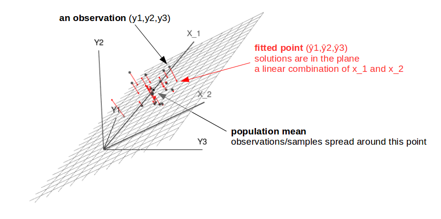
From a geometric point of view you can see regression as projection of the $n$ observations $y$ onto the surface spanned by the $m$ predictor vectors.
These observations can be seen as a point in $n$-dimensional space. The $m$ predictor vectors form a sub-space (m-dimensional, in 2 dimensions you can see it as a surface) within this $n$-dimensional space. The fitted solution of the regression is the point within this sub-space that is closest to the observation.
The image below from this question might help to see this.

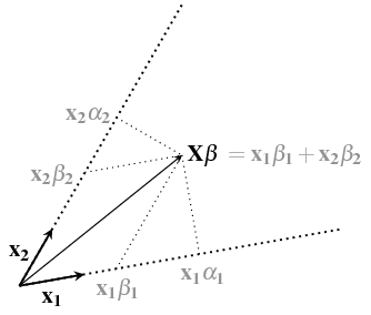
We could look perpendicular to the surface spanned by the vectors $x_1$ and $x_2$ above. The coefficients $\beta_1$ and $\beta_2$ of the solution can be seen as coordinates on this surface telling how much of vector $x_1$ and $x_2$ you need to add to get to the solution/prediction $\hat{y}$. (see the question Intuition behind $(X^TX)^{-1}$ in closed form of w in Linear Regression for an explanation of the difference between the $\alpha$ and $\beta$ coordinates in this image)

The axes of this coordinate space are however not perpendicular to each other. The following image illustrates that this creates large changes in coordinates for small changes of a point in space.

The image contains a sample of 100 randomly distributed observations/experiments as the projections/solutions of the fitting/regression. The distribution of this is a circular cloud in the case of Gaussian distributed errors.
The axes $x_1$ and $x_2$ are not perpendicular to each other but are diagonal instead. You can see that this sort of places the lines of the coordinates closer to each other (and these coordinates correspond to the coefficients that are the output of the regression). This means that the variation in this coordinate/coefficient will be larger.
The case of this graphical example is in two dimensions, but you could imagine it as extended to multiple dimensions. Multicollinearity means that at least one of the axes (corresponding to the predictor vector) has a small angle with the combination of the other axes (with the space spanned by those other axes). That means it is not necessarily one single axis and another single axis having a small angle relative to each other (in the 2D case it is), but one axis having a small angle with the subspace created by the other $m-1$ other axes.
In 3 dimensions you can view it as below. Say the axis $x_3$ is sheared and at an angle with the others. You can have this $x_3$ at a very small angle with the bottom plane of the cube (or even inside of it) without the independent angles with $x_1$ and $x_2$ being very small.

See for a related question (with many more links to other related questions) why does the same variable have a different slope when incorporated into a linear model with multiple x variables with


