convert the ATE Average Treatment Effect from a doubly robust model into Risk Ratio

Question

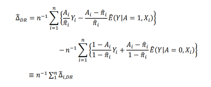
How would one convert the ATE Average Treatment Effect from a doubly robust model into Risk Ratio? Can this be done directly without having to convert to odds ratio first. If so, how is this done. Can the conversion be directly applied to the confidence intervals or would bootstrapping have to be done?

Answer 1

In the formula for the doubly robust estimator provided (augmented inverse probability weighting), it is shown for the ATE. The key piece to note is that

$$\hat{\theta}_{1} = n^{-1} \sum_{i=1}^n \frac{I(A_i=1)Y_i}{\hat{\pi}(W_i)} - \frac{A_i-\hat{\pi}(W_i)}{\hat{\pi}(W_i)} \hat{E}[Y|A=1,X_i]$$

is the estimator for the risk had everyone been given $A=1$. The second part similar follows for the risk had everyone been given $A=0$, which I indicated as $\hat{\theta}_0$. This estimator consists of 3 pieces, the inverse probability weighting part ($\frac{I(A_i=1)Y_i}{\hat{\pi}(W_i)}$), the predicted outcome ($\hat{E}[Y|A=1,X_i]$), and the 'glue' ($\frac{A_i-\hat{\pi}(W_i)}{\hat{\pi}(W_i)}$). Together these come together to estimate the risk. This form has the nice property of double robustness, but are still estimating the risk.

Once you have the two $\hat{\theta}$ or risks, you can calculate whatever contrast you prefer by manipulating those risks. For example the risk difference is just the difference in those risks (this is written out above without my $\theta$ shorthand) $$ \hat{\theta}_1 - \hat{\theta}_0$$ If you want the risk ratio, $$ \hat{\theta}_1 / \hat{\theta}_0$$ This second contrast for the risk ratio is equivalent to replacing the minus sign in the provided formula with a division.

The key piece is that the doubly robust estimator estimates each risk individually. The ATE is often frame as the estimand, so that's why it is usually presented in that form. However, the estimated risks from the doubly robust estimator can be transformed as desired.

For the estimator of the variance, influence curves are often used for the above doubly robust estimator. It is important to note that the form of the influence curve changes between the risk difference and risk ratio. Therefore, the variance estimator is a little more complicated. A simple solution is to bootstrap the variance.

Answer 2

You can split out the doubly robust estimator into two components: $$\hat \Delta_{DR} = \hat \Delta_{DR,1} - \hat \Delta_{DR,0}$$ where $$\hat\Delta_{DR,1} = \frac1n\sum_{i=1}^n \frac{Y_i}{\hat \pi_i} - \frac{A_i-\hat\pi_i}{\hat\pi_i}\hat E(Y|A = 1,X_i)$$ $$\hat\Delta_{DR,0} = \frac1n\sum_{i=1}^n \frac{Y_i}{1-\hat \pi_i} - \frac{A_i-(1-\hat\pi_i)}{1-\hat\pi_i}\hat E(Y|A = 0,X_i)$$ It is straightforward to show that (provided the substantive and regularity conditions motivating the DR estimator are true) that $\hat \Delta_{DR,1}, \hat \Delta_{DR,0}$ are separately consistent estimators of $E[Y_{i1}]$ and $E[Y_{i0}]$. Then by continuous mapping theorem, we know that $$\frac{\hat \Delta_{DR,1}}{\hat\Delta_{DR,0}}\overset p\to \frac{E[Y_{i1}]}{E[Y_{i0}]}$$ Moreover, supposing that $\hat \Delta_{DR,1}, \hat \Delta_{DR,0}$ are asymptotically normal, i.e. $$\sqrt n((\hat \Delta_{DR,1}, \hat \Delta_{DR,0})^T - \mu^T) \overset d\to \mathcal N(0,\Sigma)$$ where $\mu = (\mu_1,\mu_0) \equiv (E[Y_{i1}], {E[Y_{i0}]})$ and $\Sigma$ is the asymptotic variance matrix, then the delta method would yield $$\sqrt n\left(\frac{\hat \Delta_{DR,1}}{\hat\Delta_{DR,0}} - \frac{E[Y_{i1}]}{E[Y_{i0}]}\right)\overset d\to \mathcal N(0,g \Sigma g^T)$$ where $$g = \left(\frac{1}{\mu_0}, - \left(\frac{\mu_1}{\mu_0^2}\right)^2\right)$$ Finally, as usual, you can plug $\hat \Delta_{DR,1}, \hat\Delta_{DR,0}$ respectively for $\mu_1,\mu_0$ in the expression for $g$ and still obtain asymptotically valid inference.