Comparing percentages of samples of different sizes

Question

We compared two email sending systems and got the following results:

System 2 sample size is quite a lot smaller because it's experimental. The open rate (percentage of recipients who opened the email) is better for System 2 in all demographics except the last one. Which statistical test could be employed to determine if the improvement is statistically significant (with respect to "Open rate" for example)?

The emails assigned to System 2 were selected randomly prior to assigning them to their demographics group. All groups received the same email, and every recipient received the email at most once.

My stats memories are very rusty and, as I remember, this problem does not resemble the ones to which the t-test and chi-square test are applied.

Answer 1

You don't need any tests, just run a simple Bayesian logistic regression model:

$y_{i} \sim Binomial(1, p_{i})$

where $p_{i}$ is the probability of opening the email and $y_{i}$ is zero or one indicating whether target i has opened the email. And you model the probability with an intercept that changes according to the system being used:

$logit(p_{i}) = \alpha(System_{i})$

This is how you can fit this model using JAGS in R:

library(R2jags) # Package needed for Bayesian inference
library(boot) # Package contains the logit transform

# Some R code to simulate data 

T1 <- 160 #sample size for system 1
T2 <- 4100 #sample size for system 2
  
set.seed(123)

alpha_1 <- 0.8
alpha_2 <- 0.3

logit_p1 <- alpha_1 
logit_p2 <- alpha_2 


p1 <- inv.logit(logit_p1)
p2 <- inv.logit(logit_p2)


y1 <- rbinom(T1, 1, p1)
y2 <- rbinom(T2, 1, p2)

df1 <- data.frame(y = y1, system = 1)
df2 <- data.frame(y = y2, system = 2)
df_merged <- rbind(df1, df2)


# Jags code to fit the model to the simulated data
model_code <- "
model
{
  # Likelihood
  for (i in 1:I) {
    y[i] ~ dbin(p[i], k)
    logit(p[i]) <- alpha[system[i]]
  }
  
  # Priors
  
  for(j in 1:J){
  alpha[j] ~ dnorm(0.0,0.01)
  }

}
"

# Set up the data
model_data <- list(I = nrow(df_merged), 
                   y = df_merged$y, 
               system = df_merged$system,
                   k = 1,
                   J = 2)

# Choose the parameters to watch
model_parameters <- c("alpha")

# Run the model
model_run <- jags(
  data = model_data,
  parameters.to.save = model_parameters,
  model.file = textConnection(model_code)
)

print(model_run)

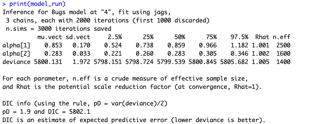
And this is the results:

You can see the full distribution estimated for $logit(p1)$ of system one ($alpha[1]$) and for $logit(p2)$ of system two ($alpha[2]$)(you can simply use $inv.logit()$ function to calculate the probability of opening the email for each). As you can see the model successfully estimated the true values (check the mean values $mu.vect$) and you can also observe the 95% CI which doesn't contain zero meaning the results are significant in frequentist terms. Note that the confidence interval associated with $alpha[1]$ is wider because you have less data on it but it doesn't matter as long as you can reasonably estimate the uncertainty (which we did) and see if you can live with that. Then increasing the sample size depends on how much risk are you willing to take.

Also you can easily expand this to incorporate different demographic groups and run the model over the whole dataset you have and give it a hierarchical structure to share information and reduce the uncertainty on the $alpha$ parameters you want to estimate without increasing the sample size.