Could any equation have predicted the results of this simulation?

Question

Suppose there is a coin that has a 5% chance of landing on HEADS and a 95% chance of landing on TAILS. Based on a computer simulation, I want to find out the following :

• The average number of flips before observing HEADS, TAILS, HEADS (note: not the probability, but the number of flips)

Using the R programming language, I tried to make this simulation (this simulation keeps flipping a coin until HTH and counts the number of flips until this happens - it then repeats this same process 10,000 times):

results <- list()

for (j in 1:10000) {

  response_i <- ''
  i <- 1

  while (response_i != 'HTH') {
    response_i <- c("H","T")
    response_i <- sample(response_i, 3, replace=TRUE, 
                         prob=c(0.05, 0.95))
    response_i <- paste(response_i, collapse = '')

    iteration_i = i
    if (response_i == 'HTH') {
      run_i = data.frame(response_i, iteration_i)
      results[[j]] <- run_i
      }
    i <- i + 1
  }
}

data <- do.call('rbind', results)

We can now see a histogram of this data:

hist(data$iteration_i, breaks = 500, main = "Number of Flips Before HTH")

We can also see the summary of this data:

summary(data$iteration_i)

   Min. 1st Qu.  Median    Mean 3rd Qu.    Max. 
    1.0   119.0   288.0   413.7   573.0  3346.0

My Question:

• Could any "mathematical equation" have predicted the results of this simulation in advance? Could any "formula" have shown that the average number of flips to get HTH would have been 413? Can Markov Chains be used to solve this problem?

• Based on the "skewed" shape of this histogram, is the "arithmetical mean" (i.e. mean = sum(x_i)/n) a "faithful" representation of the "true mean"? Looking at the above histogram, we can clearly see that you are are more likely to see HTH before 437 iterations compared to seeing HTH after 437 iterations, e.g. (on 100,000 simulations, the new average is 418):

  nrow(data[which(data$iteration_i <418), ])

63184

nrow(data[which(data$iteration_i > 418), ])

36739

For such distributions, is there a better method to find out the "expectation" of this experiment?

Thanks!

Answer 1

At any given point in the game, you're $3$ or fewer "perfect flips" away from winning.

For example, suppose you've flipped the following sequence so far: $$ HTTHHHTTTTTTH $$

You haven't won yet, but you could win in two more flips if those two flips are $TH$. In other words, your last flip was $H$ so you have made "one flip" worth of progress toward your goal.

Since you mentioned Markov Chains, let's describe the "state" of the game by how much progress you have made toward the desired sequence $HTH$. At every point in the game, your progress is either $0$, $1$, or $2$--if it reaches $3$, then you have won. So we'll label the states $0$, $1$, $2$. (And if you want, you can say that there's an "absorbing state" called "state $3$".)

You start out in state $0$, of course.

You want to know the expected number of flips, from the starting point, state $0$. Let $E_i$ denote the expected number of flips, starting from state $i$.

At state $0$, what can happen? You can either flip $H$, and move to state $1$, or you flip $T$ and remain in state $0$. But either way, your "flip counter" goes up by $1$. So: $$ E_0 = p (1 + E_1) + (1-p)(1 + E_0), $$ where $p = P(H)$, or equivalently $$ E_0 = 1 + p E_1 + (1-p) E_0. $$ The "$1+$" comes from incrementing your "flip counter".

At state $1$, you want $T$, not $H$. But if you do get an $H$, at least you don't go back to the beginning--you still have an $H$ that you can build on next time. So: $$ E_1 = 1 + p E_1 + (1-p) E_2. $$

At state $2$, you either flip $H$ and win, or you flip $T$ and go all the way back to the beginning. $$ E_2 = 1 + (1-p) E_0. $$

Now solve the three linear equations for the three unknowns.

In particular you want $E_0$. I get $$ E_0 = \left( \frac{1}{p} \right) \left( \frac{1}{p} + \frac{1}{1-p} + 1 \right), $$ which for $p=1/20$ gives $E_0 = 441 + 1/19 \approx 441.0526$. (So the mean is not $413$. In my own simulations I do get results around $441$ on average, at least if I do around $10^5$ or $10^6$ trials.)

In case you are interested, our three linear equations come from the Law of Total Expectation.

This is really the same as the approach in Stephan Kolassa's answer, but it is a little more efficient because we don't need as many states. For example, there is no real difference between $TTT$ and $HTT$--either way, you're back at the beginning. So we can "collapse" those sequences together, instead of treating them as separate states.

Simulation code (two ways, sorry for using Python instead of R):

# Python 3
import random

def one_trial(p=0.05):
    # p = P(Heads)
    state = 0 # states are 0, 1, 2, representing the progress made so far
    flip_count = 0 # number of flips so far
    while True:
        flip_count += 1
        if state == 0: # empty state
            state = random.random() < p
            # 1 if H, 0 if T
        elif state == 1: # 'H'
            state += random.random() >= p
            # state 1 (H) if flip H, state 2 (HT) if flip T
        else: # state 2, 'HT'
            if random.random() < p: # HTH, game ends!
                return flip_count
            else: # HTT, back to empty state
                state = 0

def slow_trial(p=0.05):
    sequence = ''
    while sequence[-3:] != 'HTH':
        if random.random() < p:
            sequence += 'H'
        else:
            sequence += 'T'
    return len(sequence)

N = 10**5
print(sum(one_trial() for _ in range(N)) / N)
print(sum(slow_trial() for _ in range(N)) / N)

Answer 2

First, you can refactor your R code to be (IMHO) a little more legible, also using pbapply::pbreplicate() to get a nice progress bar:

n_sims <- 1e5
library(pbapply)

results <- pbreplicate(n_sims,{
    flips <- NULL
    while(length(flips)<3 || !identical(tail(flips,3),c("H","T","H"))){
        flips <- c(flips,sample(c("H","T"),size=1,prob=c(.05,.95)))
    }
    length(flips)
})

hist(results,breaks=seq(-0.5,max(results)+0.5))

Growing the flips vector in each step makes this code very slow. It would be much faster to grow it in large batches - but that would be at the expense of legibility. As it is, this code runs its 100,000 replicates in about ten minutes, which we can use to google around a bit for an abstract solution.

Second, there indeed is an abstract solution. The details are a bit complicated, and I unfortunately don't have the time to write them all up right now, but I'll give the gist.

Specifically, we can model your sequence of unfair coin flips as a Markov chain, where each state corresponds to the last three flips, and where we stop after hitting HTH. Thus, we have a single absorbing state and seven transient states, and if we use $p$ to denote the probability of next getting a Head, we get a state transition matrix as follows:

(Apologies for pasting a picture; I don't know how to get the annotations to work in MathJaX. LaTeX code below.)

This is already in canonical form, with the single absorbing state at the bottom and the right. We can partition the matrix into a block matrix $T$ for the transient states and the row and column corresponding to the absorbing state: $$\begin{pmatrix} T & T_0 \\ 0^t & 1 \end{pmatrix}.$$

The initial states are all equally probable - this is our initial distribution $\tau$.

The distribution of the number of steps necessary to reach the absorbing state is the discrete phase-type distribution, which depends on the initial state $\tau$ and the submatrix $T$. You can take a look at Dayar (2005) on how to calculate the expectation of this distribution (also see Expected number of steps between states in a Markov Chain, where I got the pointer to this paper), but note that (1) you already start after three steps, so you would need to add $3$ to the expectation, and (2) Dayar (2005) assumes that the probability of starting in the absorbing state is zero, and in your case, it isn't, it's already $p^2(1-p)$, so you need to correct for that.

LaTeX code for the matrix, kudos to Bernard:

\documentclass{article}
\usepackage{mathtools}
\usepackage{blkarray, bigstrut}

\begin{document}

 \[ \setlength{\bigstrutjot}{4pt}
 \begin{blockarray}{r@{\enspace\vrule}rcccccccc}
   \phantom{HHH}& & HHT & HHH & THT & THH & TTT & TTH & HTT & HTH \\
  \BAhline
  \begin{block}{r@{\enspace\vrule}r(cccccccc)}
 HHT & & 0 & 0 & 0 & 0 & 0 & 0 & 1-p & p \bigstrut[t]\\
 HHH & & 1-p & p & 0 & 0 & 0 & 0 & 0 & 0 \\
 THT & & 0 & 0 & 0 & 0 & 0 & 0 & 1-p & p \\
 THH & & 1-p & p & 0 & 0 & 0 & 0 & 0 & 0 \\
 TTT & & 0 & 0 & 0 & 0 & 1-p & p & 0 & 0 \\
 TTH & & 0 & 0 & 1-p & p & 0 & 0 & 0 & 0 \\ 
 HTT & & 0 & 0 & 0 & 0 & 1-p & p & 0 & 0 \\
 HTH & & 0 & 0 & 0 & 0 & 0 & 0 & 0 & 1\bigstrut[b]\\
 \end{block}
 \end{blockarray} \]

\end{document} 

Answer 3

There is a fun way to answer this problem using martingales, and in particular using https://en.wikipedia.org/wiki/Optional_stopping_theorem. I first saw this trick in the book A First Look at Rigorous Probability Theory by Jeffrey S. Rosenthal, in the martingale chapter. (I don't have the book in front of me at the moment but I'll edit and add a page or equation number when I do.)

Imagine that at each time step $t$ a person arrives and places a bet on the outcome of the next coin toss. The payoff to their first bet is:

$\begin{equation} \begin{cases} -1 &\mbox{if toss } t \mbox{ is T} \\ +19 &\mbox{if toss } t \mbox{ is H} \\ \end{cases} \end{equation}$

If they are wrong (i.e. lose money) on this bet, they stop betting. Note that their net gain if they exit at this point is $-1$. If they are correct, they continue to betting on toss $t+1$ and receive the following payoff:

$\begin{equation} \begin{cases} +\frac{20}{19} &\mbox{if toss } t+1 \mbox{ is T} \\ -20 &\mbox{if toss } t+1 \mbox{ is H} \\ \end{cases} \end{equation}$

If they are wrong on this second bet, they stop betting. Again, note that their net gain if they exit at this point is (by design) $19-20 = -1$. If they were correct for this second bet, they proceed to betting on the outcome of toss $t+2$ and receive:

$\begin{equation} \begin{cases} -\frac{400}{19} &\mbox{if toss } t+2 \mbox{ is T} \\ +400 &\mbox{if toss } t+2 \mbox{ is H} \\ \end{cases} \end{equation}$

If they are incorrect, they exit with a net gain of $19 + \frac{20}{19} - \frac{400}{19} = -1$. If they are correct, everything stops: we have just seen a HTH sequence, and the person who started betting at the beginning of that sequence has just won $19 + \frac{20}{19} + 400 = 420.0526$.

Note that two people have started betting after this big winner: one person whose first bet was incorrect (they exit with $-1$), and a second person whose first bet was correct (they win $19$ but nothing more because the process stops).

Let $\tau$ denote the stopping time, and let $X_t$ denote the cumulative net amount won by all gamblers up to and including time $t$. Let $X_0 = 0$, and note that $X_t$ is a martingale because all bets are (by construction) fair, with an expected payoff of $0$. This will let us use https://en.wikipedia.org/wiki/Optional_stopping_theorem and in particular $\mathbf{E}[X_\tau] = \mathbf{E}[X_0] = 0$.

$X_\tau$ is the total amount won when we reach the stopping time. At this point $\tau - 3$ people will have lost their bets and exited with a net gain of $-1$, one person will have won $420.0526$, and we also have to account for the last two people who start betting after the winner. We have:

$\begin{equation} \mathbf{E}[X_\tau] = 0 = (\mathbf{E}[\tau]-3)*(-1) + 420.0526 + (-1) + 19 \end{equation}$

Which leads to $\mathbf{E}[\tau] = 420.0526 + 3 + 18 = 441.0526$, which agrees with the answers posted earlier.

Answer 4

Here is a somewhat clumsy brute-force method to obtain the probabilities and order statistics. Getting the mean will take more work.

So first just generate the possible sequences and associated probabilities where "HTH" are the last 3 flips (with that sequence not occurring previously). Then look for patterns. For integer patterns the go to place is http://oeis.org.

Note: To make some of the calculations easier I've used 1 for H and 0 for T. Using Mathematica the probabilities for the flip that ends with "HTH" (or "101") with general $p$ is generated as follows:

s[1] = {{1, 0, 1}};
pr[1] = p^2 (1 - p);
Print[{1, pr[1]}]
Do[s[i] = Select[Flatten[{Prepend[#, 1], Prepend[#, 0]} & /@ s[i - 1], 1], ! (#[[1]] == 1 && #[[2]] == 0 && #[[3]] == 1) &];
 pr[i] = Total[p^Total[#] (1 - p)^(Length[#] - Total[#]) & /@ s[i]],
 {i, 2, 8}]
Table[{i, pr[i]}, {i, 1, 8}] // TableForm

The pattern of the powers of $p$ and $1-p$ seems obvious but maybe not the associated coefficients. That's where http://oeis.org comes in. We plug in the coefficients for $n=8$

1,6,12,13,9,6,1,1

and find sequence A124279. That translates to the formula for the probability of flip $n$ ending in "HTH" (and not containing any previous "HTH" sequence):

pr[n_] := p^2 (1 - p) Sum[p^(n - k - 1) (1 - p)^k Sum[Binomial[j, k - j] Binomial[n - k - 1, k - j], {j, 0, n}], {k, 0, n - 1}]

or

$$pr(n) = p^2 (1-p) \sum _{k=0}^{n-1} (1-p)^k p^{-k+n-1} \sum _{j=0}^n \binom{j}{k-j} \binom{-k+n-1}{k-j}$$

The median is between flip 303 and 304 as the associated cumulative probabilities are 0.49891 and 0.500051, respectively, when $p=0.05$.

To calculate the probabilities in R you'll either need to use multiple precision arithmetic or reduce round-off errors by using logs.

Answer 5

Disclosure: I wrote the samc R package used in this answer

This answer is more of a supplement to Stephan Kolassa's answer

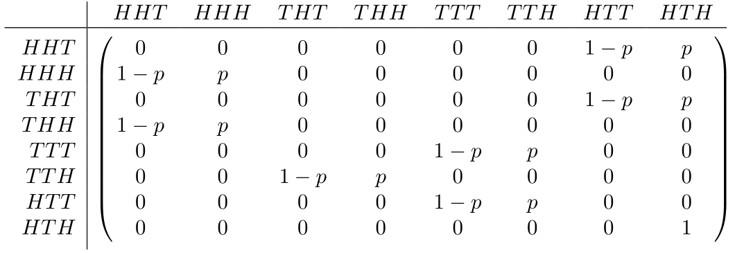
In it, he showed how to construct a transition matrix representing the problem: Image credit: Stephan Kolassa's answer

Now, as indicated in comments/another answer, this matrix can be simplified a variety of different ways, but I'm going to keep it as-is because there are other things about the experiment you can learn from it that you can't from the others.

Let's call this transition matrix $P$, which is how I define it in the samc package: samc overview

This can be broken down as: $$ P = \begin{bmatrix} Q & R \\ 0 & I \end{bmatrix} $$

Using this, there a variety of things you can calculate about the model. For example: $$z=(I-Q)^{-1}{\cdot}1=F{\cdot}1$$ Will tell you the expected time to absorption given a starting transient state. In this example, that means that given your last 3 flips, how many more flips do you expect it to take before $HTH$ occurs. Some code:

library(samc)

p <- 0.05
q <- 1 - p

p_mat <- matrix(c(0, 0, 0, 0, 0, 0, q, p,
                  q, p, 0, 0, 0, 0, 0, 0,
                  0, 0, 0, 0, 0, 0, q, p,
                  q, p, 0, 0, 0, 0, 0, 0,
                  0, 0, 0, 0, q, p, 0, 0,
                  0, 0, q, p, 0, 0, 0, 0,
                  0, 0, 0, 0, q, p, 0, 0,
                  0, 0, 0, 0, 0, 0, 0, 1),
                8, byrow = TRUE)

rownames(p_mat) <- c("HHT", "HHH", "THT", "THH", "TTT", "TTH", "HTT", "HTH")
colnames(p_mat) <- c("HHT", "HHH", "THT", "THH", "TTT", "TTH", "HTT", "HTH")

# A samc object is the core of the package
samc_obj <- samc(p_mat)

# Given the last 3 flips, how many more flips until we hit HTH (absorption)?
survival(samc_obj)
[1] 420.0000 421.0526 420.0000 421.0526 441.0526 421.0526 441.0526

So, if we start with $HHT$, we expect it would take 420 flips on average to end up with $HTH$. $THT$ is the same, and they represent the best case scenario where we start only one flip away from $HTH$. Conversely, $TTT$ and $HTT$ are a worst case scenario where we start off needing 3 perfect flips; the result for these is 441.0526, the same as other answers.

As Neil Slater pointed out in a comment, the transition matrix can be reduced to 5 elements if this all you want. But there are other metrics to explore. For example, we can calculate the number of times we expect a sequence to occur before we hit $HTH$:

$$F = (I-Q)^{-1}$$

Here's some code (I include some code to show the relationship to the previous metric as well):

# Given a starting point (in this case, a sequence of 3 flips), how many times
# would we expect the different combinations of 3 flips to occur before absorption?
visitation(samc_obj, origin = "HHT")
[1]   1.95   0.05  18.05   0.95 361.00  19.00  19.00

sum(visitation(samc_obj, origin = "HHT")) # Compare to survival() result
[1] 420

# Instead of a start point, we can look at an end point and how often we expect
# it to occur for each of the possible starting points
visitation(samc_obj, dest = "THT")
[1] 18.05 18.05 19.05 18.05 19.00 19.00 19.00

# These results are just rows/cols of a larger matrix. We can get the entire matrix
# of the start/end possibilities but first we have to disable some safety measures
# in place because this package is designed to work with extremely large P matrices
# (millions of rows/cols) where these types of results will consume too much RAM and
# crash R
visitation(samc_obj)
Error: This version of the visitation() method produces a large dense matrix.
See the documentation for details.

samc_obj$override <- TRUE
visitation(samc_obj)
     [,1]       [,2]  [,3] [,4] [,5] [,6] [,7]
[1,] 1.95 0.05000000 18.05 0.95  361   19   19
[2,] 1.95 1.10263158 18.05 0.95  361   19   19
[3,] 0.95 0.05000000 19.05 0.95  361   19   19
[4,] 1.95 0.10263158 18.05 1.95  361   19   19
[5,] 1.00 0.05263158 19.00 1.00  381   20   19
[6,] 1.00 0.05263158 19.00 1.00  361   20   19
[7,] 1.00 0.05263158 19.00 1.00  380   20   20

rowSums(visitation(samc_obj)) # equivalent to survival() above
[1] 420.0000 421.0526 420.0000 421.0526 441.0526 421.0526 441.0526

Another one: $$D=(F-I)diag(F)^{-1}$$ would calculate the probability of a sequence of flips occurring before you hit $HTH$. And there's a "short-term" version of this: $$\tilde{D}_{jt}=(\sum_{n=0}^{t-1}\tilde{Q}^n)\tilde{q}_j$$ which calculates the same thing, but within a given number of time steps (or coin flips in this context). So let's say you're interested in the probability of flipping $TTT$ with only 3 flips:

dispersal(samc_obj, dest = "TTT", time = 3)
[1] 0.902500 0.857375 0.902500 0.857375       NA 0.857375 0.950000

Depending on your last 3 flips, you basically have 3 options (4 if you count having already flipped $TTT$): $0.95$, $0.95^2=0.9025$, or $0.95^3= 0.857375$.

Obviously, some of these things can be easier or more intuitive to calculate using other methods, but once set up, absorbing markov chains give you a lot of flexibility in exploring a scenario.

A full list of the things you can calculate (at least using my package) are available in the function reference: samc functions. Which calculations are relevant depends on the context. When writing the functions, I used the book “Finite Markov Chains” by Kemeny and Snell as reference, which includes proofs. You can find the pdf of it online for free (legally, I believe) pretty easily.

Tying things back to OP's questions: as the other answers have shown, there are a variety of ways to mathematically model your experiment, including Markov chains. One thing Stephen Kolassa alluded to, and what I was hoping to show, is there is a LOT more you can learn about this experiment than you might have realized.

Note: the package was originally written for spatial applications, so a lot of the terminology in it is biased towards that. However, it is usable for pretty much any application of absorbing Markov chains

Answer 6

Seems very close to Shannon - related theorems. If you posit "HTH" as your "end of message" string, you want to estimate the chance that "HTH" shows up in random data. I suspect a little digging into his work will provide the equations/ formulas of interest.

And because I can't resist, "HTH"

Answer 7

Final formula appears to be

sum(i = 1 to length(pattern) : if (first i flips of pattern match the last i flips of pattern) then P(series of i flips matches first i flips of pattern)^-1 else 0)

(For a fair coin, this reduces to Conway's algorithm; it can probably be proven by a similar method.)