How well do power calculations actually work in reality?

Question

I'm planning a study and I need to do a power calculation. So much of it seems to depend on guesswork and estimations of what the data (that I don't have yet) will look like. Guesswork seems to be such standard practice I can't help but wonder how accurate they are in practice. Does anyone know of a study that's compared predicted power against association rate?

e.g. of all the studies claiming they will 90% power to detect an association at p<0.05, what percentage actually find an association at p<0.05 when they get the data and that prediction hits the real world? Is it close to 90?

This is purely curiosity driven, I understand the need for a power calculation, I'm just curious how well they actually work across science.

Answer 1

1. You don't know when $H_0$ is false, so you can't compute the correct empirical rejection rate for power from looking at the results of tests. You shouldn't include the cases where the null was true in that calculation. (If you could say when $H_0$ was false, you wouldn't need tests in the first place.)

   Further, even if you could tell when $H_0$ was true or false, it would still be wrong. Unless you worked with a whole power curve across effect sizes, desired power was specified at some given population effect size. The sample equivalent is the proportion of correct rejections at that population effect size, so the denominator would be limited to the number of comparable cases where the effect was actually that size (which of course you don't know).

2. That said, power calculations are based on your requirements in relation to the population -- what's the minimum power you require at some meaningful population effect size -- e.g. it might be an effect that is clinically important or educationally relevant (e.g. the power you want if the effect was a 5% higher pass rate on some skills test, say), and so forth -- an amount you would be interested in having good power at.

   What is an effect size of interest does not typically come from data. It is not a statistical consideration, but a subject matter one. To this end it's usually better (where possible; for some variables this won't be the case) to frame such considerations in terms of raw effects rather than standardized effects, since it's on the scale of raw effects that such considerations would typically apply. It is also not likely to be a matter of just a few moments thought (for all that this often seems to be all it's accorded from what I have seen); it also requires solid domain knowledge to understand what such an effect size might be.

3. There's a tendency I've seen to base power calculation inputs on the estimated effects from some previous study. There's often no obvious reason why a noisy estimate of a population effect size should be an effect size at which you want some given power -- this is conflating two distinct tasks, with distinct considerations.

   However, if one were to use estimates of quantities like (say) an estimate of a population mean and standard deviation, it would be quite wrong to treat those as if they were the population values. This practice will lead to typically lower power than the usual (population-based) calculations suggest, and sometimes much less. One appropriate way to investigate this (particularly for more complicated models) would be via simulation.

Answer 2

You can view a typical power calculation not as guess work, but as an estimate of the unknown fixed true power. This means you can also perform inference on power by constructing a confidence interval for it using parameter estimates and standard error estimates from historical studies. In the example below the point estimate of power is above 90% but the inference cannot rule out that the true power might be considerably lower.

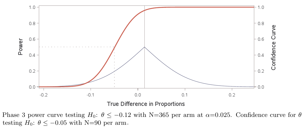
Example: A phase 2 and 3 development plan is being created for an asset to treat an immuno-inflammation disorder. Phase 3 is planned as a non-inferiority study using a difference in proportions on a binary responder index. The non-inferiority margin is set by the regulatory agency at –0.12, as is the one-sided significance level of 0.025. Phase 2 is a dose finding study on a continuous endpoint. This study also collects data on the responder index and includes a control arm to estimate the difference in proportions planned for phase 3. A stricter non-inferiority margin of –0.05 is considered in phase 2, but since the sample size in phase 2 is typically smaller than in phase 3, a larger one-sided significance level of 0.20 is tolerated. Based on a literature review the estimated response proportion for the comparator is 0.43 with N=1200.

The power curve shows the long-run probability of succeeding in phase 3 as a function of the unknown true difference in proportions based on N=365 subjects per arm when testing Ho: Difference in Proportions ≤ –0.12 at the one-sided 0.025 significance level using a likelihood ratio test. This long-run probability forms the level of confidence in the next experimental outcome. If one is satisfied with the inference on phase 3 power given minimal success in phase 2, one would be satisfied for any other successful phase 2 result. The confidence curve above depicts one-sided p-values and confidence intervals of all levels by inverting a likelihood ratio test, showing what minimal success would look like at the end of phase 2. This is based on N=90 subjects per arm, a 0.43 response rate estimate in the control arm, and an estimated difference in proportions of 0.01 (minimum detectable effect) testing Ho: Difference in Proportions ≤ –0.05. This produces a one-sided p-value of 0.20. A nearly identical confidence curve can be produced by inverting a Wald test using an identity link function. The p-value depicts the ex-post sampling probability of the observed phase 2 result or something more extreme if the hypothesis for the difference in proportions is true. This long-run probability represents the plausibility of the hypothesis given the data.

The figure above shows that minimal success in phase 2 produces inference around high values of phase 3 power, but still assumes some risk. While the maximum likelihood estimate of phase 3 power is 95.9%, one can claim with only 80% confidence that the power of the phase 3 study is no less than 50% given minimal success in phase 2 (p-value = 0.2 testing Ho: Phase 3 Power ≤ 0.50). The phase 2 null hypothesis Ho: Difference in Proportions ≤ –0.05 was chosen as the value at which phase 3 power is 50%.

In my view ensuring phase 3 power is no worse than a coin toss conditional on passing phase 2 is a good rule of thumb. If stronger inference on phase 3 power is desired given minimal success in phase 2, one could simply increase the phase 3 sample size. This will steepen the phase 3 power curve relative to the phase 3 null hypothesis by lowering the phase 3 minimum detectable effect. Alternatively, one could adjust the phase 2 significance level and null hypothesis, and select the phase 2 sample size based on an acceptable phase 2 minimum detectable effect. Once the phase 2 study results are available, two-sided confidence limits for phase 3 power can be provided along side the maximum likelihood point estimate. These point and interval estimates can even be plotted as a function of the phase 3 sample size.

Here is a paper that discusses performing inference on power and compares this to Bayesian probability of success. Here is a related LinkedIn article.

Answer 3

To answer this question, it is useful to first separate the power function itself from sample-size calculations that try to achieve a stipulated level of power against an alternative hypothesis. The power function arises whenever we have a proposed method of hypothesis testing and it measures the probability of rejecting the null hypothesis in the test, conditional on the true value of the parameter under analysis. The power function is a function of the parameter of interest in the test, the significance level for the test, and the sample size. However, it does not depend on the data values --- just the sample size.

Now, when we undertake sample-size calculations on the basis of a power requirement, we need to stipulate three things: (1) the significance level for the test; (2) the minimum level of power we want to achieve; and (3) the (alternative) parameter value against which we wish to achieve this level of power. Once we stipulate these three things, there is some minimum sample size $n$ that will achieve the required level of power against the stipulate value of the parameter. There is no guesswork of what the data will look like here, because the content of the data are not required for this computation.

As to the idea of undertaking empirical tests to do a post hoc check of the power, the only thing that is really worth checking is whether or not the underlying model assumptions for the test are accurate or not. If the underlying model assumptions are accurate then the power calculation is accurate --- it merely reflects a mathematical property of the test under that model. If an empirical assessment of the power curve were to examine the rejection rate in studies, it would need to know the true parameter values in those studies to know where on the power curve it is supposed to be comparing the empirical rejection rates to.