Linear algebra shows
$$2(x_4(x_1-x_3)+x_5(x_2-x_1)) =(x_2-x_3+x_4+x_5)^2/4-(-x_2+x_3+x_4+x_5)^2/4+\sqrt{3}(-\sqrt{1/3}x_1+\sqrt{1/12}(x_2+x_3)+(1/2)(-x_4+x_5))^2-\sqrt{3}(-\sqrt{1/3}x_1+\sqrt{1/12}(x_2+x_3)+(1/2)(x_4-x_5))^2.$$
Each squared term is a linear combination of independent standard Normal variables scaled to have a variance of $1,$ whence each of those squares has a $\chi^2(1)$ distribution. The four linear combinations are also orthogonal (as a quick check confirms), whence uncorrelated; and because they are uncorrelated joint random variables, they are independent.
Thus, the distribution is that of (a) half the difference of two iid $\chi^2(1)$ variables plus (b) $\sqrt{3}$ times half the difference of independent iid $\chi^2(1)$ variables.
(Differences of iid $\chi^2(1)$ variables have Laplace distributions, so this equivalently is the sum of two independent Laplace distributions of different variances.)
Because the characteristic function of a $\chi^2(1)$ variable is
$$\psi(t) = \frac{1}{\sqrt{1-2it}},$$
the characteristic function of this distribution is
$$\psi(t/2) \psi(-t/2) \psi(t\sqrt{3}/2) \psi(-t\sqrt{3}/2) = \left[(1+t^2)(1+3t^2)\right]^{-1/2}.$$
This is not the characteristic function of any Laplace variable -- nor is it recognizable as the c.f. of any standard statistical distribution. I have been unable to find a closed form for its inverse Fourier transform, which would be proportional to the pdf.
Here is a plot of the formula (in red) superimposed on an estimate of $\psi$ based on a sample of 10,000 values (real part in black, imaginary part in gray dots):

The agreement is excellent.
Edit
There remain questions of what the PDF $f$ looks like. It can be computed by numerically inverting the Fourier Transform by computing
$$f(x) = \frac{1}{2\pi}\int_{\mathbb R} e^{-i x t} \psi(t)\,\mathrm{d}t = \frac{1}{2\pi}\int_{\mathbb R} \frac{e^{-i x t}}{\sqrt{(1+t^2)(1+3t^2)}}\,\mathrm{d}t.$$
This expression, by the way, fully answers the original question. The aim of the rest of this section is to show it is a practical answer.
Numerical integration will become problematic once $|x|$ exceeds $10$ or $15,$ but with a little patience can be accurately computed.
In light of the analysis of differences of Gamma variables at https://stats.stackexchange.com/a/72486/919, it is tempting to approximate the result by a mixture of the two Laplace distributions. The best approximation near the middle of the distribution is approximately $0.4$ times Laplace$(1)$ plus $0.6$ times Laplace$(\sqrt{3}).$ However, the tails of this approximation are a little too heavy.

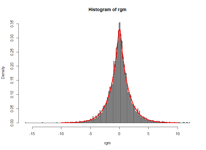
The left hand plot in this figure is a histogram of 100,000 realizations of $x_4(x_1-x_3) + x_5(x_2-x_1).$ On it are superimposed (in black) the numerical calculation of $f$ and then, in red, its mixture approximation. The approximation is so good it coincides with $f.$ However, it's not perfect, as the related plot at right shows. This plots $f$ and its approximation on a logarithmic scale. The decreasing accuracy of the approximation in the tails is clear.
Here is an R function for computing values of a PDF that is specified by its characteristic function. It will work for any numerically well-behaved CF (especially one that decays rapidly).
cf <- Vectorize(function(x, psi, lower=-Inf, upper=Inf, ...) {
  g <- function(y) Re(psi(y) * exp(-1i * x * y)) / (2 * pi)
  integrate(g, lower, upper, ...)$value
}, "x")
As an example of its use, here is how the black graphs in the figure were computed.
f <- function(t) ((1 + t^2) * (1 + 3*t^2)) ^ (-1/2)
x <- seq(0, 15), length.out=101)
y <- cf(x, f, rel.tol=1e-12, abs.tol=1e-14, stop.on.error=FALSE, subdivisions=2e3)
The graph is constructed by connecting all these $(x,y)$ values.
This calculation for $101$ values of $|x|$ between $0$ and $15$ takes about one second. It is massively parallelizable.
For more accuracy, increase the subdivisions argument--but expect the computation time to increase proportionally. (The figure used subdivisions=1e4.)


