Calculate uncertainty of the slope when dependent variable in a linear regression has substantial error?

Question

I have a dataset in which the dependent variable (y) has known and substantial error, and yet the observations happen to line up quite well along a line when plotted against the independent variable (x). Fitting a linear regression seems to substantially overestimate the precision of the slope estimate for y vs. x.

How can one appropriately propagate the known error in y through to the estimate of the slope?

I think there is part of an answer here, but it assumes the point fit a linear regression exactly: Calculate uncertainty of linear regression slope based on data uncertainty

As a reproducible example in R:

# the data
set.seed(5)
dat <- data.frame(x = 0:8, y = seq(0,16, length.out=9)+rnorm(9, 0, 0.5), y.se = 3)

# fit a naive model, not considering error in y
mod <- lm(y ~ x, dat)
summary(mod)
preds <- predict(mod, se.fit = TRUE)

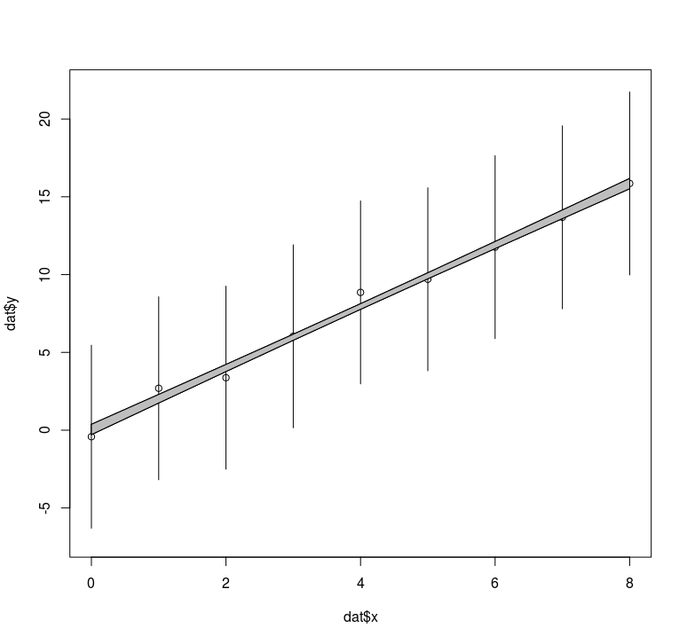
plot(dat$x, dat$y, ylim=c(-7,22))
arrows(dat$x, dat$y-1.96*dat$y.se, dat$x, dat$y+1.96*dat$y.se, length=0)

# plot the confidence interval on the linear regression
polygon(c(dat$x, rev(dat$x)), c(preds$fit+preds$se.fit, rev(preds$fit-preds$se.fit)), col = 'grey')

The slope is estimated very precisely near 2.0:

Coefficients:
            Estimate Std. Error t value Pr(>|t|)    
(Intercept)  0.04670    0.32783   0.142    0.891    
x            1.97546    0.06886  28.689 1.61e-08 ***

Visually, however, a slope as low as 0.7 or as high as 3.3 would still fit through the error bounds of y quite well.

Answer 1

This can be handled with structural equation modelling (SEM)

library(lavaan)

code = '
yhat ~ x     # Latent variable predicted by x
yhat =~ 1*y  # y is the single indicator of yhat
y ~~ 9*y     # y has error variance of 9 (3^2)
'

fit = lavaan(code, dat)
summary(fit)

lavaan 0.6-7 ended normally after 3 iterations

  Estimator                                         ML
  Optimization method                           NLMINB
  Number of free parameters                          1
                                                      
  Number of observations                             9
                                                      
Model Test User Model:
                                                      
  Test statistic                                24.572
  Degrees of freedom                                 1
  P-value (Chi-square)                           0.000

Parameter Estimates:

  Standard errors                             Standard
  Information                                 Expected
  Information saturated (h1) model          Structured

Latent Variables:
                   Estimate  Std.Err  z-value  P(>|z|)
  yhat =~                                             
    y                 1.000                           

Regressions:
                   Estimate  Std.Err  z-value  P(>|z|)
  yhat ~                                              
    x                 1.975    0.387    5.101    0.000

Variances:
                   Estimate  Std.Err  z-value  P(>|z|)
   .y                 9.000                           
   .yhat              0.000   

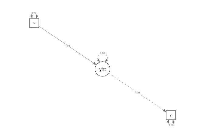
Plots can also be useful...

library(semPlot)
semPaths(fit, what = 'path', whatLabels = 'est', layout = 'circle2')

Answer 2

I'm not quite sure what your problem actually is. If there's random error in y but not x, the regression of y on x will be unbiased. The uncertainty due to the error will be properly reflected in the standard error of the parameter estimate.

In your example, the y.se variable is only used to draw the "arrows" in the graph. It's not used to calculate y, so it's not reflected in the lm results. Your y and x are almost perfectly correlated (r>.99), so one can predict the other almost perfectly.