Which statistical test to use (repeated measures ANOVA?)

Question

I am a student conducting a clinical trial for my thesis. We have two independent variables: (1) time point (pre-test, post-test) and (2) control v. experimental group.

We'll be measuring about 6 or 7 continuous outcome variables (repeated measures at times one and two) to see if the experimental group benefits from the intervention.

I'm pretty rusty in statistics at this point and could use a starting point.

Answer 1

Yes, you could use repeated measures Anova (RMA). HOWEVER, but I would suggest to use mixed effects models with patient id as random effects instead (RMA is a type of mixed effects models). See this answer here going into more detail: https://stats.stackexchange.com/a/237294/343024.

To demonstrate how I would proceed here in R, let's assume your response is y, you have independent variables Time (pre, post) and Group (Control, Treat). All study participants have a unique id and have y recorded at both pre and post:

Create the dataset dd:

dd<-data.frame(id=rep(c(1:6000),2),
               Time=rep(c("pre","post"), each=6000),
               Group=rep(rep(c("Treat","Control"),2), each=3000),
               y=c(rnorm(3000,90,5), rnorm(3000,87,5), rnorm(3000,70,5), rnorm(3000,88,5)))

Make pre reference level:

dd$Time=relevel(as.factor(dd$Time), ref="pre")

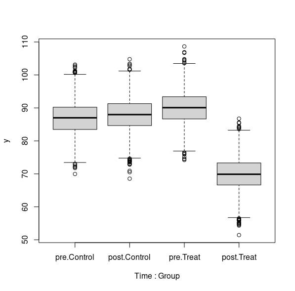
Plot your data:

par(mfrow=c(1,1))
boxplot(y~Time+Group, dd)

Now fit the repeated measures Anova:

maov<- aov(y ~ Group*Time + Error(id), dd)
summary(maov)

Error: id
      Df Sum Sq Mean Sq
Group  1 125676  125676

Error: Within
              Df Sum Sq Mean Sq F value              Pr(>F)    
Group          1  40480   40480    1635 <0.0000000000000002 ***
Time           1 272975  272975   11029 <0.0000000000000002 ***
Group:Time     1 336772  336772   13606 <0.0000000000000002 ***
Residuals  11995 296894      25

As you can see, your response y differs (P<0.0001) for variables Group, Time, and in particular the interaction term Group:Time (indicating that y changes differently between Control and Treat).

Now we can fit a mixed effects model using R-paclage lme4:

me1<-lmer(y~Time+Group+Group:Time+(1|id), dd)
summary(me1)

Linear mixed model fit by REML ['lmerMod']
Formula: y ~ Time + Group + Group:Time + (1 | id)
   Data: dd

REML criterion at convergence: 72568.4

Scaled residuals: 
    Min      1Q  Median      3Q     Max 
-3.9053 -0.6769  0.0024  0.6698  3.7353 

Random effects:
 Groups   Name        Variance Std.Dev.
 id       (Intercept)  0.00    0.000   
 Residual             24.75    4.975   
Number of obs: 12000, groups:  id, 6000

Fixed effects:
                     Estimate Std. Error  t value
(Intercept)          86.91326    0.09083  956.880
Timepost              1.05620    0.12845    8.222
GroupTreat            3.15322    0.12845   24.548
Timepost:GroupTreat -21.19032    0.18166 -116.648

You can see straight away from:

1. the coefficient for Time, that your response y in Control (reference level in variable Group) increased by 1.05620 from pre (reference level in variable Time) to post
2. the coefficient for Group, that your response y in Treat at reference-Time pre was 3.15322 higher than in Control
3. the change from pre to post in Treat was 21.19032 lower than Control, which is your difference of interest between both groups.

Be aware that per default, R-package lme4 does not provide p-values (for good reasons). However, there are ways to obtain them by using for example package lmerTest:

library(lmerTest)
anova(me1)
Type III Analysis of Variance Table with Satterthwaite's method
           Sum Sq Mean Sq NumDF DenDF F value                Pr(>F)    
Time       272975  272975     1 11996   11029 < 0.00000000000000022 ***
Group      166147  166147     1 11996    6713 < 0.00000000000000022 ***
Time:Group 336772  336772     1 11996   13607 < 0.00000000000000022 ***