8 out of 10 Cats - Optimal Sample

Question

I was watching a lecture earlier by Marcus du Sautoy called: 'Thinking Better with Mathematics.'

Marcus discusses the statistical sample sizes to verify statements about the population. In his own example, he addresses a statement about cat food.

In particular, a cat food brand in the 1970s/80s argued that "8 out of 10 cats preferred this cat food."

The population size (in the UK) at that time was 7 million. But to verify this statement, only a relatively small sample of 246 would be required.

The statement from that video is: For a population of 7 million cats, if we sample 246 cats, then 19 out of 20 times the sample is within 5% of the true value.

I wondered if someone could derive this, given the the limited information? Or if not, provide a link/direction on this type of information.

The video lecture with the information is here at 13:30 to 15:20 mins. https://www.youtube.com/watch?v=4PlmsnyWXMw

Answer 1

Because the variance of a binomial distribution depends on the success probability $p,$ one must be specific about the null and alternative values of $p$ in order to find the power of an exact binomial test of $H_0: p = p_0$ against $H_a: p = p_a.$

One experiment:

Suppose you have $p_0 = 0.4, p_a = 0.5, n = 246.$ For one performance of the experiment, we reject $H_0$ at the 0.2% level of significance. Exact binomial test in R:

set.seed(2021)
x = rbinom(1, 246, .5); x
x/246
[1] 0.5

binom.test(x, 246, p=.4)

   Exact binomial test

data:  x and 246
number of successes = 123, number of trials = 246, p-value = 0.001731
alternative hypothesis: 
true probability of success is not equal to 0.4
95 percent confidence interval:
     0.4358163 0.5641837
sample estimates:
 probability of success 
     0.5 

Simulated power:

To approximate the power of the test, we look at the proportion of rejections among 100,000 performances of the experiment. The power is about 89%.

n = 246; p.0 = .4; p.a = .5
set.seed(405)
pv = replicate(10^5, binom.test(rbinom(1,n,p.a), n, p=p.0)$p.val)
mean(pv <+ .05)
[1] 0.8863

However, $n = 246$ would give power about 96% distinguishing between $p_0 = 0.8$ and $p_a = 0.7,$ because binomial distributions have less variability for these relatively large success probabilities (or for relatively small ones).

n = 246; p.0 = .8; p.a = .7
set.seed(406)
pv = replicate(10^5, binom.test(rbinom(1,n,p.a), n, p=p.0)$p.val)
mean(pv <+ .05)
[1] 0.95787

---

Note: Various statistical software programs have 'power and sample size' procedures. Here is output from a recent release of Minitab, to find the sample sizes required to get 95% power for $p_0 = 0.8, p_a = 0.75$ and for $p_0 = 0.8, p_a = 0.75,$ for tests that use normal approximations to binomial distributions. (Of course somewhat larger samples are required for 96% power as in my simulation.)

Power and Sample Size 

Test for One Proportion

Testing p = 0.8 (versus < 0.8)
    α = 0.05

                  Sample  Target
    Comparison p    Size   Power  Actual Power
            0.75     751    0.95      0.950008
            0.70     200    0.95      0.950561

Answer 2

I could not verify the statement

For a population of 7 million cats, if we sample 246 cats, then 19 out of 20 times the sample is within 5% of the true value.

Trying to reverse engineer what they might have done, we could have

$$\frac{0.8}{\sqrt{246}} \approx 0.05$$

But that expression makes no sense.

Another potential derivation, mentioned by Whuber in the comments, could be based on a z-test but with a minor mistake.

$$ Z_{\alpha/2} \cdot \sigma_X = 0.05 \cdot \mu_X $$

Filling in the variance $\sigma_X = \sqrt(np(1-p)$ and mean $\mu_X = pn$ of the binomial distribution gives an answer close to the computation below. But if one fills in $\mu_X = n$, then the result will be $n \approx 246$. That is however an erroneous computation.

---

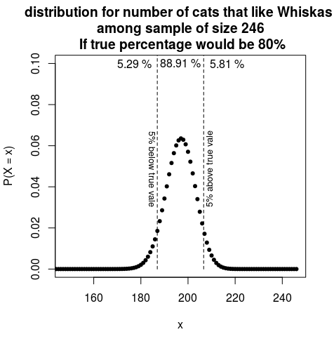
Say, the true probability is 0.8 and you sample 246, then the outcome of your experiment will be binomial distributed (given that you performed the experiment well like sampling independently and without bias as mentioned in the video).

Below is a plot how this distribution looks like and what the probability is to be 5% of the true value.

So, if the true value would be 80% then there is a 11.09 % probability that the observed percentage in the sample would be more than 5% away from the true value.

---

Note that this is only one way to make the computation. The computation of the interval that contains the true value 95% of the time (19 out of 20 cases), also known as a confidence interval can be done in different ways (by using different approaches or viewpoints). For the estimate of a percentage/proportion, the different ways are summarized on this Wikipedia page: https://en.wikipedia.org/wiki/Binomial_proportion_confidence_interval

But in any case, the number of 246 seems too low (although it is not a large difference, with the method that created the image the correct size would be $n=367$).

---

R-code to make the figure:

### settings
n = 246
#n = 367
p = 0.8
q = 1-p
x = 0:n

### plot binomial distribution
plot(x,dbinom(x,n,p), xlim = c(n*0.6,n), 
     pch = 21, col = 1, bg = 1, cex = 0.7, ylim = c(0,0.1),
     ylab = "P(X = x)", xlab = "x", main = "distribution for number of cats that like Whiskas \n among sample of size 246 \n If true percentage would be 80%")

### add upper and lower 5% boundaries
upper = n*p*1.05
lower = n*p*0.95
lines(upper * c(1,1), c(0,1), lty = 2)
lines(lower * c(1,1), c(0,1), lty = 2)
text(upper, 0.03, "5% above true vale", pos = 4, srt = 90, cex = 0.8)
text(lower, 0.03, "5% below true vale", pos = 2, srt = -90, cex = 0.8)


### compute percentages and add to plot
x3 = round((1-pbinom(upper, n, p))*100,2)
x1 = round((pbinom(lower, n, p))*100,2)
x2 = round(100 - (1-pbinom(upper, n, p))*100 - (pbinom(lower, n, p))*100,2)

text(n*p, 0.1, paste0(x2, " %"))
text(n*p*1.1, 0.1, paste0(x3, " %"))
text(n*p*0.9, 0.1, paste0(x1, " %"))