10
$\begingroup$

What would a bayesian do if she wanted to do inference for the mean with a large sample but has no idea of the underlying distributions?

A frequentist statitician would use the sample mean as a point estimate and CLT for the distribution of the estimator. All she has to assume is finite variance.

I have found Bernstein Von-Mises Theorem which states that given a random sample $X_1, \ldots, X_n$ and

  • a prior $p(\mu)$ for the mean
  • a distribution for the sample given the parameter $f_{x | \mu}$

Then if the sample size is sufficiently large the posterior distribution of the mean given the sample is approximately normal, i.e

$$ \mu_{|_{X_1, \ldots X_n}} \approx \mathcal{N}\left( \hat{\mu}_{ml}\, ; \, \frac{1}{I(\mu_0) n}\right)$$

Where the mean is the maximum likelihood estimator and $I(\mu_0)$ is Fisher information number for the true mean.

In the case where we have no knowledge of $f_{x | \mu}$ there is the problem that maximum likelihood nor fisher information number can be calculated. But what can be done? Becuase even if we do not know it the distribution exists and it will be approximately normal.


Intentions:

Some buisness woman has to take an action based on the true sign of the mean. A decision has to be made so she will use the sign of the sample mean but she needs some measure of the potential cost that arise in case of making the wrong decistion.

So, if the sample mean is positive things like

$$ P\left( \mu < 0 | X_1 \ldots X_n \right) = \int_{-\infty}^0 f_{\mu |x_1 \ldots x_n}( t) \, dt.$$ or

$$ E \left( \mu I_{(-\infty, 0)}| X_1 \ldots X_n \right) = \int_{-\infty}^0 t f_{\mu |x_1 \ldots x_n}( t) \, dt.$$
would make a lot of (buisness) sense for her.

In the frequentist context she is stuck with affirmations of the kind: With $95\%$ confidence the mean is greater than a certain value.

$\endgroup$
4
  • 1
    $\begingroup$ i am not sure what your question is. But maybe you are after a bayesian CLT? see stat.columbia.edu/~gelman/book/BDA3.pdf pages 587... $\endgroup$
    – seanv507
    Commented Apr 5, 2022 at 21:15
  • 8
    $\begingroup$ Given that there is no information beyond the (large) sample, one would think that even the most Bayesian Bayesian would just calculate the sample mean... What do you really want to know? $\endgroup$ Commented Apr 5, 2022 at 21:17
  • 1
    $\begingroup$ @MichaelLew i have added some detail of my intention hope it helps. $\endgroup$
    – Manuel
    Commented Apr 6, 2022 at 13:04
  • 3
    $\begingroup$ In fact the mean is quite non-robust in a frequentist sense. If the underlying distribution has heavy tails, even with existing variance, the sample size at which the CLT provides a good approximation may be arbitrarily large, i.e. larger than any sample size you may have. (Bayesians should worry about this as well.) $\endgroup$ Commented Apr 6, 2022 at 13:49

4 Answers 4

8
$\begingroup$

With a Bayesian method we could also consider $\bar{X} = \frac{1}{n} \sum_{k=1}^n X_k$ as the observed statistic and it has approximately a normal distribution if we assume that the values have finite variance and converges quickly.

So we could use the likelihood function $\mathcal{L}(\mu \vert \bar{X}) \approx \frac{1}{\sqrt{2 \pi \sigma^2/n}} \exp \left(\frac{(\bar X - \mu)^2}{2 \sigma^2/n} \right)$

Then we still need priors for $\sigma$ and $\mu$ but that is like any other Bayesian problem. The issue with the likelihood has been solved by assuming a normal distribution just like with the frequentist method.

Related question: Would you say this is a trade off between frequentist and Bayesian stats?

$\endgroup$
4
  • 1
    $\begingroup$ This is what i need. It did take me some time to realize that $\mathcal{L}(\mu | \bar X) = f( \bar X | \mu)$. The related question was quite helpful. Thanks! $\endgroup$
    – Manuel
    Commented Apr 6, 2022 at 16:53
  • 1
    $\begingroup$ I am struggling to give $\mathcal{L}(\mu , \sigma^2 | \bar X, S^2)$ any idea o how should that be? $\endgroup$
    – Manuel
    Commented Apr 7, 2022 at 13:11
  • 1
    $\begingroup$ @Manuel in my answer the $S^2$ is not included as observation. We just have $\mathcal{L}(\mu , \sigma^2 | \bar X)$ $\endgroup$ Commented Apr 7, 2022 at 17:39
  • 1
    $\begingroup$ You could add $S^2$ as well but then you are gonna relate to assuming some specific type of probability distribution, which you wanted to avoid. $\endgroup$ Commented Apr 7, 2022 at 17:41
8
$\begingroup$

There are various flavours of Bayesian statistics. One of them is subjectivist (e.g., according to de Finetti). Subjectivist Bayesians hold that probability applies to an individual's state of belief and information but not to underlying data generating processes, which can never be infinitely repeated, which would be necessary to define a true frequentist probability. For this reason (and potentially some others that are harder to discuss), according to a subjectivist, there is no such thing as a true underlying distribution. So the job of the subjective Bayesian in this problem is not to guess the underlying distribution, but rather to specify a distribution that summarises her belief and knowledge about the expected distribution of the data given $\mu$. Not only $p(\mu)$ is a prior choice, also what you call $f_{x|\mu}$!

In fact, this is even the case in what many call "objectivist Bayes", as long as the probabilities are epistemic, i.e., do refer to a state of knowledge rather than really existing underlying data generating processes. The objectivist also will have to choose an $f_{x|\mu}$ that expresses all existing information about the expected distribution of the data given $\mu$ (except that subjective belief is not supposed to play a role here; although in reality it is often hard to bring existing information into a suitable formal form without any subjective choices).

These are the major streams of traditional Bayesian philosophy. In the present, much of Bayesian data analysis is based on an implicit assumption that there is a true underlying distribution, which we have called "falsificationist Bayes" here: https://rss.onlinelibrary.wiley.com/doi/10.1111/rssa.12276

Even here (as in frequentism), the task would be to specify a model that makes sense from a subject matter perspective, and that can then be checked, for example by comparing data generated from it with your actual data, as in so-called posterior predictive checks (hence "falsificationist").

There is also the field of Bayesian nonparametrics, which is about very large models with potentially infinite-dimensional parameters covering large sets of the model space in case you don't want to commit to a specific simple one. This may be relevant regardless of whether your probability model is interpreted in an epistemic or frequentist (underlying data generating process) sense.

$\endgroup$
1
  • 1
    $\begingroup$ Thanks for all this info. It is really interesting. $\endgroup$
    – Manuel
    Commented Apr 6, 2022 at 16:54
4
$\begingroup$

You're essentially asking if you can do Bayesian statistics without a likelihood function. The answer is no. The likelihood function is an essential ingredient in Bayesian statistics. Without a likelihood, you have no way to update your prior.

If you can't specify a likelihood, or are unable to evaluate it, you can use approximate Bayesian computation to sample from the posterior. This still requires specifying a likelihood, but it's a working likelihood that you know isn't correct.

$\endgroup$
1
  • 1
    $\begingroup$ abc still uses a likelihood function or at least some statistical model that describes the probability of the data given the parameters. The idea behind it is that the computation of the likelihood is too difficult (because of nuisance parameters) or the computation of the posterior is too difficult, and is being approximated with sampling. $\endgroup$ Commented Apr 6, 2022 at 14:10
4
$\begingroup$

You seem to be asking about a nonparametric estimator for the mean.

First, let's make it clear: for Bayesian statistics, you always need to make distributional assumptions. You can proceed as suggested by Sextus Empiricus (+1), but this does assume Gaussian distribution. If you really didn't want to make any assumptions, in practice, you would probably just estimate the arithmetic mean.

But let's try coming up with a nonparametric solution. One thing that comes to my mind is Bayesian bootstrap also described by Rasmus Bååth who provided code example. With Bayesian bootstrap, you would assume the Dirichlet-uniform distribution for the probabilities, resample with replacement the datapoints and evaluate the statistic, so arithmetic mean on those samples. But in such a case, to approximate the frequentist estimator, you would use the same estimator on the samples to find their distribution. Not very helpful, isn't it?

Let's start again. The definition of expected value is

$$ E[X] = \int x \, f(x)\, dx $$

The problem is that you don't know the probability densities $f(x)$. With the parametric model, you would solve it by finding a parametric distribution for $f$. In the frequentist setting, we would estimate the expected value using the arithmetic average with $\phi_i$ weights equal to the empirical probabilities

$$ \widehat{E[X]} = \sum_{i=1}^N x_i \, \phi_i $$

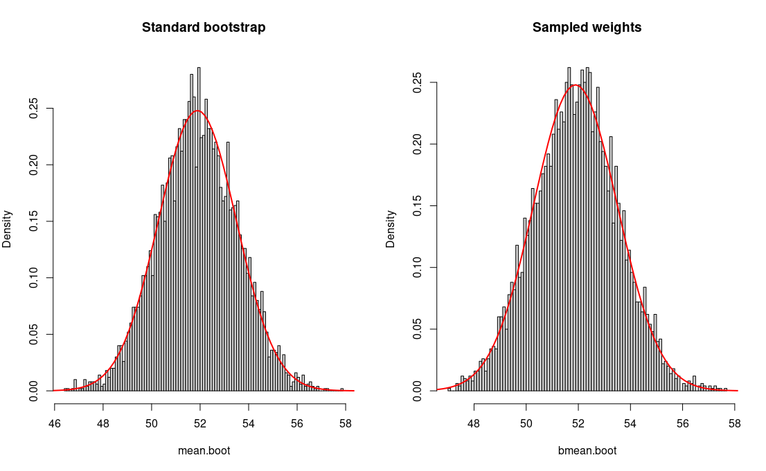
Same as with Bayesian bootstrap, you could assume a prior Dirichlet-uniform prior for the $\phi_i$ weights, sampling the weights, calculating the weighted average, and repeating this many times to find the distribution of the estimates. If you think about it, It's the most trivial case of the Bayesian bootstrap for a weighted statistic. Yes, this makes a number of unreasonable assumptions like approximating continuous distribution with a discrete one. It's also not necessarily very useful, but if you insist on a Bayesian nonparametric estimator, that's a possibility. As you can see from the example below, it gives the same results as the frequentist estimator and standard bootstrap.

set.seed(42)

N <- 500
X <- rnorm(N, 53, 37)
mean(x)
## [1] 51.88829

R <- 5000
mean.boot <- replicate(R, mean(sample(X, replace=TRUE)))
summary(mean.boot)
##    Min. 1st Qu.  Median    Mean 3rd Qu.    Max. 
##   46.41   50.81   51.90   51.91   53.03   57.88 

# weighted.mean itself normalizes the weights
wmean.boot <- replicate(R, weighted.mean(X, w=rexp(N, 1)))
summary(wmean.boot)
##    Min. 1st Qu.  Median    Mean 3rd Qu.    Max. 
##   47.09   50.82   51.93   51.91   52.99   57.65 

par(mfrow=c(1, 2))

hist(mean.boot, 100, freq=FALSE, main="Standard bootstrap")
curve(dnorm(x, mean(X), sd(X)/sqrt(N)), 45, 60, add=T, col="red", lw=2)

hist(wmean.boot, 100, freq=FALSE, main="Sampled weights")
curve(dnorm(x, mean(X), sd(X)/sqrt(N)), 45, 60, add=T, col="red", lw=2)

Standard bootstrap vs the described solution are the same as frequentist estimate for the sampling distribution.

In the end, it's the same as the frequentist estimator, so you could just use the frequentist estimator.

$\endgroup$

Your Answer

By clicking “Post Your Answer”, you agree to our terms of service and acknowledge you have read our privacy policy.

Not the answer you're looking for? Browse other questions tagged or ask your own question.