3
$\begingroup$

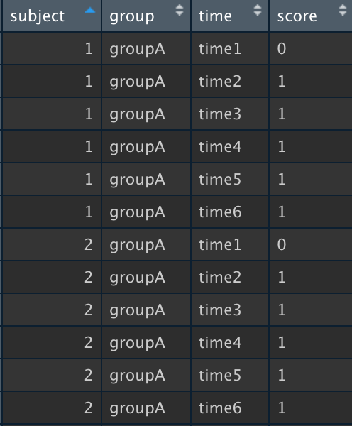
I'm new here and my question might be a bit long. Sorry in advance. I want to analyze two groups of patients in repeated measures, and to investigate whether there is a significant difference over time between groups. My data consist of one dependent variable (dichotomous- 0/1) and two independent variables (group: A,B and time: time1, time2,...time6).

enter image description here

I used the generalized linear mixed model, and the results are as follows:

data2$group <- relevel(data2$group, ref = "groupA") 
data2$time <- relevel(data2$time, ref = "time1") 
model <- glmer(score ~ time * group + (1 | subject), data = data2, family = binomial("logit"), control = glmerControl(optimizer = "bobyqa"), nAGQ = 0)
summary(model, correlation = FALSE)

Fixed effects:
                       Estimate Std. Error z value Pr(>|z|)    
(Intercept)             -1.5469     0.4135  -3.741 0.000183 ***
timetime2                2.0747     0.4826   4.299 1.71e-05 ***
timetime3                3.9292     0.6081   6.462 1.03e-10 ***
timetime4                4.7745     0.7422   6.433 1.25e-10 ***
timetime5                5.9804     1.1096   5.390 7.06e-08 ***
timetime6                5.9804     1.1096   5.390 7.06e-08 ***
groupgroupB             -0.5176     0.6253  -0.828 0.407803    
timetime2:groupgroupB    1.7377     0.7613   2.282 0.022461 *  
timetime3:groupgroupB    1.2571     0.9841   1.277 0.201426    
timetime4:groupgroupB    0.8736     1.1528   0.758 0.448542    
timetime5:groupgroupB   15.9771  1397.4011   0.011 0.990878    
timetime6:groupgroupB   15.9771  1397.4011   0.011 0.990878    
---
Signif. codes:  0 ‘***’ 0.001 ‘**’ 0.01 ‘*’ 0.05 ‘.’ 0.1 ‘ ’ 1

I deduce the following from the result: With reference Group A and Time 1 point, the score changes over time and there is no difference between groups; however, time * group interaction is significant.

My questions are:

  1. Is the conclusion I stated above correct?
  2. When I use car::Anova , there is no time * group interaction. Is it wrong to do the following analysis? What's the difference between them?
Anova(model, type = 3)
Response: score
              Chisq Df Pr(>Chisq)    
(Intercept) 13.9981  1   0.000183 ***
time        83.3778  5  < 2.2e-16 ***
group        0.6852  1   0.407803    
time:group   5.3224  5   0.377808    
---
Signif. codes:  0 ‘***’ 0.001 ‘**’ 0.01 ‘*’ 0.05 ‘.’ 0.1 ‘ ’ 1
  1. Is post hoc analysis necessary? Is it binary comparison if I look for significance by changing the references with relevel? For example with time : group command:
data2$group <- relevel(data2$group, ref = "groupB") 
data2$time <- relevel(data2$time, ref = "time4") 
model <- glmer(score ~ time : group + (1 | subject), data = data2, family = binomial("logit"), control = glmerControl(optimizer = "bobyqa"), nAGQ = 0)
summary(model, correlation = FALSE)

Fixed effects:
                       Estimate Std. Error z value Pr(>|z|)    
(Intercept)              0.5278     0.3703   1.425 0.154025    
timetime4:groupgroupB    3.0559     0.8696   3.514 0.000442 ***
timetime3:groupgroupB    2.5941     0.7605   3.411 0.000648 ***
timetime1:groupgroupB   -2.5923     0.5976  -4.338 1.44e-05 ***
timetime6:groupgroupB   19.3653  1397.4007   0.014 0.988943    
timetime5:groupgroupB   19.3653  1397.4007   0.014 0.988943    
timetime2:groupgroupB    1.2201     0.5764   2.117 0.034274 *  
timetime4:groupgroupA    2.6998     0.7079   3.814 0.000137 ***
timetime3:groupgroupA    1.8545     0.5675   3.268 0.001083 ** 
timetime1:groupgroupA   -2.0747     0.4826  -4.299 1.71e-05 ***
timetime6:groupgroupA    3.9057     1.0864   3.595 0.000324 ***
timetime5:groupgroupA    3.9057     1.0864   3.595 0.000324 ***

In this analysis, time2:groupA is dropping. So can I say this: Group A is significant different in the Time 2 point than Group B?

  1. If above mentioned commands wrong, is this post-hoc analysis true in below? Can I use emm function to compare binomial variables? Or is it only appropriate for continuous data? It is stated that it can be used in many R articles, but I am not sure. In this analysis, Group A is not differ in the Time 2 point than Group B.
summary(glht(model, emm(pairwise ~ time * group)), test=adjusted(type="holm"))

Linear Hypotheses:
                                   Estimate Std. Error z value Pr(>|z|)    
time1 groupA - time2 groupA == 0 -2.075e+00  4.826e-01  -4.299 0.000874 ***
time1 groupA - time3 groupA == 0 -3.929e+00  6.081e-01  -6.462 6.52e-09 ***
time1 groupA - time4 groupA == 0 -4.775e+00  7.422e-01  -6.433 7.78e-09 ***
time1 groupA - time5 groupA == 0 -5.980e+00  1.110e+00  -5.390 3.81e-06 ***
time1 groupA - time6 groupA == 0 -5.980e+00  1.110e+00  -5.390 3.81e-06 ***
time1 groupA - time1 groupB == 0  5.176e-01  6.253e-01   0.828 1.000000    
time1 groupA - time2 groupB == 0 -3.295e+00  6.050e-01  -5.446 2.84e-06 ***
time1 groupA - time3 groupB == 0 -4.669e+00  7.825e-01  -5.967 1.43e-07 ***
time1 groupA - time4 groupB == 0 -5.131e+00  8.889e-01  -5.772 4.55e-07 ***
time2 groupA - time2 groupB == 0 -1.220e+00  5.764e-01  -2.117 1.000000 
.....
.....
  1. Last one:) May I compare the groups in this way:
model_postHoc <- glmer(score ~ group + (1 | subject), data = data2[data2$time == "time2", ], family = binomial("logit"), control = glmerControl(optimizer = "bobyqa"), nAGQ = 0)
summary(model_postHoc, correlation = FALSE)

Random effects:
 Groups  Name        Variance  Std.Dev. 
 subject (Intercept) 2.329e-12 1.526e-06
Number of obs: 104, groups:  subject, 104

Fixed effects:
            Estimate Std. Error z value Pr(>|z|)  
(Intercept)   0.4700     0.2850   1.649   0.0992 .
groupgroupB   1.0940     0.4643   2.356   0.0185 *
---
Signif. codes:  0 ‘***’ 0.001 ‘**’ 0.01 ‘*’ 0.05 ‘.’ 0.1 ‘ ’ 1

In this analyze, there is a difference between the groups in the Time 2 point. I am confused. I am aware that this method can be reduced the statistical power, and increase Type 1 error.

Thanks in advance.

$\endgroup$
12
  • $\begingroup$ There is something weird about your data: Why are the coefficients for time 5 and time 6 the same for both groups A and B? Also see huge the standard errors for time 5 and time 6 in group B. I wouldn't be making conclusions before fixing this. $\endgroup$
    – dipetkov
    Commented Jun 10, 2022 at 22:27
  • $\begingroup$ @dipetkov thanks for the comment. The dependent variable is a count variable (like yes or no). It is because the number of cases with the same degree was also equal at time 5 and time 6 (in group A: 51 yes, 1 no in both times; in group B: 52 yes, 0 no in both times). In terms of the standard errors, I can't comment because my statistical knowledge is not sufficient to interpret this; sorry. $\endgroup$
    – Ertan
    Commented Jun 10, 2022 at 22:47
  • $\begingroup$ I want to edit the comment. The dependent variable was determined by whether a subject could perform a test or not. $\endgroup$
    – Ertan
    Commented Jun 10, 2022 at 22:58
  • $\begingroup$ Of course, complete separation! High p-values for logistic regression variable that perfectly separates? $\endgroup$
    – dipetkov
    Commented Jun 10, 2022 at 23:47
  • $\begingroup$ @dipetkov thanks for the answer and reference. I read the reference, and Frank Harrell suggest using likelihood ratio tests in such cases. I analyzed the model with the Type III Wald chisquare tests. Is that wrong you think? $\endgroup$
    – Ertan
    Commented Jun 11, 2022 at 0:20

1 Answer 1

0
$\begingroup$

After my research and consulting with some statisticians, I would like to answer my question and open my answer for discussion.

Since there is a categorical variable with more than two levels (time1, time2,.., time6), it is difficult to interpret the results with the summary() function as @gungReinstateMonica answered a question in here. For example, in the result below, result of timetime2:groupgroupB present that additional difference between groupB and groupA when time2 OR additional difference between time2 and time1 when groupB (reference). But I am mainly interested in the interaction between group and time. Maybe pairwise comparisons can be made regardless of whether the interaction is significant or not; however, I am not sure (please interpret this inference). So, I think, summary() function cannot be an option for my purpose. Thus, the third, fourth, and fifth propositions are also disabled.

data2$group <- relevel(data2$group, ref = "groupA") 
data2$time <- relevel(data2$time, ref = "time1") 
model <- glmer(score ~ time * group + (1 | subject), data = data2, family = binomial("logit"), control = glmerControl(optimizer = "bobyqa"), nAGQ = 0)
summary(model, correlation = FALSE)

Fixed effects:
                       Estimate Std. Error z value Pr(>|z|)    
(Intercept)             -1.5469     0.4135  -3.741 0.000183 ***
timetime2                2.0747     0.4826   4.299 1.71e-05 ***
timetime3                3.9292     0.6081   6.462 1.03e-10 ***
timetime4                4.7745     0.7422   6.433 1.25e-10 ***
timetime5                5.9804     1.1096   5.390 7.06e-08 ***
timetime6                5.9804     1.1096   5.390 7.06e-08 ***
groupgroupB             -0.5176     0.6253  -0.828 0.407803    
timetime2:groupgroupB    1.7377     0.7613   2.282 0.022461 *  
timetime3:groupgroupB    1.2571     0.9841   1.277 0.201426    
timetime4:groupgroupB    0.8736     1.1528   0.758 0.448542    
timetime5:groupgroupB   15.9771  1397.4011   0.011 0.990878    
timetime6:groupgroupB   15.9771  1397.4011   0.011 0.990878    
---
Signif. codes:  0 ‘***’ 0.001 ‘**’ 0.01 ‘*’ 0.05 ‘.’ 0.1 ‘ ’ 1

I think, I should analyze the model with car::Anova [Anova(model, type = 3, test.statistic = "Chisq")] (References: answer of @RussLenth in here and Dr. Jacob Wobbrock in sixty-sixth page). The result is:

Analysis of Deviance Table (Type III Wald chisquare tests)

Response: score
              Chisq Df Pr(>Chisq)    
(Intercept) 23.5614  1   1.21e-06 ***
group         0.1194  1     0.7296    
time       83.3778  5  < 2.2e-16 ***
group:time   5.3224  5     0.3778    
---
Signif. codes:  0 ‘***’ 0.001 ‘**’ 0.01 ‘*’ 0.05 ‘.’ 0.1 ‘ ’ 1

As a result, I conclude that there is no interaction between group and time. And, if desired, post hoc analysis for the time variable can be performed with a created a new model without the interaction as follows:

model2 <- glmer(score ~ group + time + (1|subject), data = data2, family = binomial("logit"), control = glmerControl(optimizer = "bobyqa"), nAGQ = 0)
summary(glht(model2, emm(pairwise ~ time)), test = adjusted(type = "bonferroni"))

OR

emmeans(model2, pairwise ~ time, adjust = "bonferroni", mode = "linear.predictor", type = "Score")

I would be very grateful if you could review my answer and give your comments. Thanks in advance.

$\endgroup$

Your Answer

By clicking “Post Your Answer”, you agree to our terms of service and acknowledge you have read our privacy policy.

Not the answer you're looking for? Browse other questions tagged or ask your own question.