influence of bayesian priors: rjags and categorical variables

Question

I am a bad statistician and new using Bayesian tools, and I am learning how to make regressions with rjags. While toying, I came across a situation I do not fully understand, and I would need some help from the community.

the example:

library(data.table)
library(ggplot2)
library(rjags)
library(magrittr)

global_slope <- 1
global_intercept <- 1

Npoints_per_group <- 50
N_groups <- 10
pentes <- rnorm(N_groups,-1,.5)

centers_x <- seq(0,10,length = N_groups)
center_y <- global_slope*centers_x + global_intercept

group_spread <- 2
group_names <- sample(LETTERS,N_groups)

df <- lapply(1:N_groups,function(i){
  x <- seq(centers_x[i]-group_spread/2,centers_x[i]+group_spread/2,length = Npoints_per_group)
  y <- pentes[i]*(x- centers_x[i])+center_y[i]+rnorm(Npoints_per_group)
  data.table(x = x,y = y,ID = group_names[i])
}) %>% rbindlist()

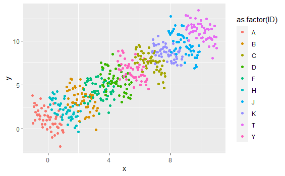
It creates a dataset with a classical Simpson paradox:

ggplot(df,aes(x,y,color = as.factor(ID)))+
  geom_point()

I can use mixed effect regression, but in a first step I just wanted to perform a regression adjusted for the ID categorical variable:

lm(y ~ x + ID,data = df) %>% summary()

lm(formula = y ~ x + ID, data = df)

Residuals:
    Min      1Q  Median      3Q     Max 
-3.1638 -0.7172 -0.0060  0.6544  2.9827 

Coefficients:
            Estimate Std. Error t value Pr(>|t|)    
(Intercept)  3.32405    0.16884  19.687   <2e-16 ***
x           -0.99256    0.07785 -12.750   <2e-16 ***
IDG         17.79467    0.72174  24.655   <2e-16 ***
IDH          8.88795    0.40220  22.098   <2e-16 ***
IDN         15.26829    0.63928  23.884   <2e-16 ***
IDS         -2.05924    0.22256  -9.252   <2e-16 ***
IDT         11.07778    0.47865  23.144   <2e-16 ***
IDU          2.11935    0.22256   9.522   <2e-16 ***
IDW         13.28410    0.55804  23.805   <2e-16 ***
IDY          4.20289    0.26829  15.665   <2e-16 ***
IDZ          6.61491    0.33074  20.000   <2e-16 ***

Now I want to do the same with rjags. I do the following:

model_code <- 
"model
{
  
  for (i in 1:n) {
    y[i] ~ dnorm(mu[i], sigma^-2)
    mu[i] <- alpha + beta * x[i] + bID[ID[i]]
  }
  
  # cat distrib
  bID[1] <- 0
  for(j in 2:Nid){
  bID[j] ~ dunif(-5,5)
  }
  
  # Priors
  alpha ~ dnorm(0, 100^-2)
  beta ~ dnorm(0, 100^-2)
  sigma ~ dunif(0, 10)
}
"


df[,ID_num := as.numeric(as.factor(ID))]
model_data <- list(n = nrow(df), 
                   Nid = df[,uniqueN(ID)],
                   ID = df$ID_num,
               y = df$y, 
                   x = df$x)

model <- jags.model(textConnection(model_code),
                    data = model_data,
                    n.chains = 2,
                    n.adapt = 1000)
update(model, 1000)

samples <- coda.samples(    model,
    c("alpha", "beta", "sigma","bID"),
    1000)

summary(samples)

This does not give the expected results:

1. Empirical mean and standard deviation for each variable,
   plus standard error of the mean:

            Mean      SD  Naive SE Time-series SE
alpha    2.38553 0.20216 0.0045205       0.023001
bID[1]   0.00000 0.00000 0.0000000       0.000000
bID[2]   4.94015 0.05910 0.0013216       0.003490
bID[3]   2.45937 0.22747 0.0050864       0.009988
bID[4]   4.42102 0.24729 0.0055295       0.012415
bID[5]  -1.11753 0.27499 0.0061490       0.022423
bID[6]   3.17433 0.23565 0.0052692       0.011053
bID[7]   0.09581 0.24132 0.0053960       0.014685
bID[8]   3.90678 0.25029 0.0055967       0.012346
bID[9]   0.71809 0.23663 0.0052912       0.012584
bID[10]  1.66045 0.23142 0.0051747       0.011332
beta     0.33399 0.02955 0.0006607       0.003277
sigma    1.31688 0.04148 0.0009275       0.001146

I realized that it was because the prior I gave for the categorical variable ID is too narrow. If I replace

bID[j] ~ dunif(-5,5)

by

bID[j] ~ dunif(-100,100)

in the JAGS model, then I find results similar to those of the frequentist lm:

1. Empirical mean and standard deviation for each variable,
   plus standard error of the mean:

          Mean      SD  Naive SE Time-series SE
alpha    3.292 0.16957 0.0037918      0.0194214
bID[1]   0.000 0.00000 0.0000000      0.0000000
bID[2]  17.622 0.66571 0.0148857      0.2021913
bID[3]   8.805 0.35826 0.0080109      0.0892269
bID[4]  15.123 0.57542 0.0128667      0.1739097
bID[5]  -2.025 0.22548 0.0050420      0.0194497
bID[6]  10.969 0.43419 0.0097089      0.1219498
bID[7]   2.107 0.21089 0.0047156      0.0170001
bID[8]  13.156 0.51186 0.0114454      0.1450026
bID[9]   4.165 0.24613 0.0055036      0.0381072
bID[10]  6.545 0.29735 0.0066490      0.0548702
beta    -0.972 0.07282 0.0016284      0.0193806
sigma    1.027 0.03268 0.0007307      0.0009942

So the question:

I was expecting that even if the priors are wrong or too narrow (my bID[j] ~ dunif(-5,5)), the model would at the end converge to the expected solution if it has enough iterations, as each step posterior distribution os based on the data. But it seems it does not. The MCMC seems to have converged (to the wrong result), and increasing the number of burning does not alter the result.

Why is that ? Do the priors constrain the possible results whatever the number of iterations ? Or is there a kind of local minima reached before the actual true result ?

Answer 1

If you set as a prior for the ID coefficients a uniform distribution between -5 and 5, this means that these coefficients are assumed to be in the interval $[-5,5]$, other values are impossible. These cannot become possible during the MCMC algorithm, because you have specified these values as a priori impossible. As the frequentist analysis estimates these values outside that interval, the Bayesian analysis will necessarily deviate quite a bit from the frequentist one.

The way you generated the data implies (as confirmed by the frequentist analysis) that there are so big differences between the ID means that $[-5,5]$ is not enough of a range to fit them. In other words, choosing the prior like this actively prevents the Bayesian analysis from finding the "correct" coefficient values. This is no longer the case for a uniform on $[-100,100]$.

By the way, also the priors for alpha and beta look very restrictive, even though the normal distribution at least doesn't make any value totally impossible. In a proper Bayesian analysis you need to choose the priors so that they allow the data to have enough influence to put the parameters anywhere where they could realistically occur. Overprecision in the priors is not good.