4
$\begingroup$

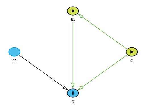
I am working with DAGs as a way to do some causal modeling. I am using dagitty - both the website and the R package. I feel like I have a good grasp of most things related to confounding, adjustment sets, and so on. However, something has me confused. Let me demonstrate by example.

Assume I have the DAG enter image description here

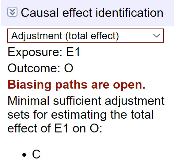
I understand (and dagitty confirms) that to extract a causal value for E1 I need to adjust for C. Dagitty reports "

dagitty adjustment set

So, for example, if everything was linear, I would build a model O ~ E1 + C, and I would intepret the coefficient of E1 as causal. I understand that I cannot interpret C as causal - this would violate the "Table 2 Fallacy".

Now for the part that confuses me. Dagitty allows a user to pick multiple exposures. So, for example, I can choose both E1 and C as "exposures".

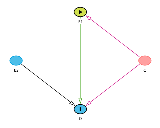
enter image description here

Dagitty now tells me that "No adjustment is necessary to estimate the total effect of E1,C on O." This would seem to suggest that the same model: O ~ E1 + C can be used, but now ?both? E1 and C have casual meaning. Obviously, this is wrong.

My question is - what is the meaning of "the total effect of E1,C"? Since C causes E1 (by my diagram) I can't set them independently. More generally, what is the meaning of any multiple exposure selection. In other words, let's say I had the DAG E1 -> O <- E2. What would be the meaning of setting both E1 and E2 as exposures?

Thanks in advance for any explanations. Every time I think I have my head wrapped around causal inference, some new "wrinkle" pops up.

$\endgroup$

1 Answer 1

5
$\begingroup$

The problem is the same estimation procedure you used in the first case, cannot be used in the second.

DAG 1:

In the first case, you rely on a very special case where the average causal effect (ACE) can be estimated. Specifically, if (1) the outcome is continuous, (2) the true model specification has not interaction terms, and (3) a single exposure; then the coefficient for $E1$ can be interpreted as the ACE for $E1$ on $O$. As you say, trying to interpret the coefficient for $C$ leads to the Table 2 Fallacy.

A more general approach (i.e., it works when the outcome is not continuous or when there are interaction terms) is g-computation. Briefly, we would estimate the outcome model as suggested. Then we would manually set $E1 = 1$ in a copy of the data set and use the fitted model to predict $O$ for everyone with $E1$. This process would then be repeated for $E1=0$. Then we would take the mean of those predictions under each set $E1$ and then subtract. This gives us the ACE while allowing for more complex models. Furthermore, it prevents the Table 2 Fallacy by only providing the ACE as the output.

DAG 2:

Now in the second example, you try to use the linear regression trick but it won't work in this case. There are now two exposures that we are setting. Specifically, we may want to estimate the ACE had everyone been given $E1=1,C=1$ versus had everyone been given $E1=0,C=0$. The linear regression coefficients cannot give you these comparisons (since they condition on the other). Trying to interpret these issues again would end up with the Table 2 Fallacy. However, the problem is not in the identification but it is in the estimation approach you are using.

Instead, you can use the g-computation procedure. After estimating the model (as done before), you would now set both $E1$ and $C$ then generate the predicted values. Therefore, the problem is not in identification (daggity is correct in saying the causal effects are identifiable) but is a problem in the estimation strategy (since it is a special case that doesn't apply in the latter).

From a graphical perspective. The $C \rightarrow E1$ in the second DAG doesn't mean much. In our intervention (on both exposures), we are setting both $E1$ and $C$. By setting both, $C$ would no longer be predictive of $E1$ (e.g., we are setting $E1 = 1$ under our intervention and it doesn't depend on the value of $C$).

$\endgroup$
4
  • 1
    $\begingroup$ thank you very much for the detailed reply. I do have a follow-up. In your explanation, you describe (using the g-computation approach) "setting both E1 and C". This (rather than the linear regression part - which turned out to be a distraction) was my main source of confusion. If, as posited, C -> E1, then an intervention where we are "setting both E1 and C" seems to violate the causal structure of the system. $\endgroup$
    – MikeS
    Commented May 6, 2022 at 14:55
  • $\begingroup$ The causal structure of the system in DAG 2 is like what happens out in the world (i.e., observational data). This DAG is distinct from a DAG that represents application of the intervention on the system. Under you intervention, you are setting E1 and C from outside the system, so there would be no input arrows from other variables (for the ACE). DAG 2 tells you whether you can identify the effect of that intervention given the observational data (i.e., it does not represent the intervention itself) $\endgroup$
    – pzivich
    Commented May 6, 2022 at 15:08
  • $\begingroup$ Hello @pzivich. I'm recently discovered DAGs and I'm confused. What do you mean by "estimation" and "identification" ? Thanks. $\endgroup$ Commented May 28 at 21:16
  • $\begingroup$ Hi @Boussens-DumonGrégoire the distinction I am drawing here is the DAG tells you the independencies that hold in your causal structure that allow you to write the parameter of interest in terms of the observations (i.e., identification). However, that does not give your the recipe of how to actually estimate the quantity you are interested in. The following paper might help with drawing the distinction further arxiv.org/abs/2108.11342 $\endgroup$
    – pzivich
    Commented May 29 at 14:04

Your Answer

By clicking “Post Your Answer”, you agree to our terms of service and acknowledge you have read our privacy policy.

Not the answer you're looking for? Browse other questions tagged or ask your own question.