Does Neyman-Pearson Lemma consider the case when the likelihood ratio equals the critical value?

Question

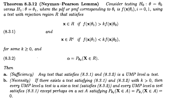
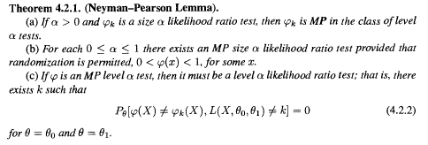
Here are three different versions of Neyman-Pearson lemma. They differ in that the first two (books) ignore the case when the likelihood ratio equals the critical value, while the last one (Wikipedia) doesn't. I feel not ignoring is natural, because ignoring will leave the set where the likelihood ratio equals the critical value to be undecided. So I was wondering why some ignore while some don't? Thanks and regards!

1. In Casella and Berger's Statistical Inference

2. In Bickel and Doksum's Mathematical Statistics Vol 1

   

   Especially in (c), the event excludes the case when the likelihood ratio $L(x, \theta_0, \theta_1)$ equals the critical value $k$. So how can we say the $\phi_k$ ahd $\phi$ are equivalent up to a set of probability zero?

3. In Wikipedia:

   when performing a hypothesis test between two point hypotheses $H_0: θ = θ_0$ and $H_1: θ = θ_1$, then the likelihood-ratio test which rejects $H_0$ in favour of $H_1$ when $$ \Lambda(x)=\frac{ L( \theta _0 \mid x)}{ L (\theta _1 \mid x)} \leq \eta $$ where $$ P(\Lambda(X)\leq \eta\mid H_0)=\alpha $$ is the most powerful test of size $α$ for a threshold $η$.

Answer 1

Perusal of the derivation of the existence part of the Neyman-Pearson lemma in $\rm [I], ~[II]$ will show that the test function $\varphi(\mathbf x) $ takes $\gamma$ when $f(\mathbf x|\theta_1) =cf(\mathbf x|\theta_0). $ This warrants an elaboration: let $f(\mathbf x|\theta_1)/f(\mathbf x|\theta_0)\equiv \mathrm Y; ~\mathbb P_{\theta_0}(\mathrm Y> c) =: \alpha(c).~\alpha(\cdot)$ is non-increasing, right continuous and $$\mathbb P_{\theta_0} (\mathrm Y=c) = \alpha(c^{-})-\alpha(c).\tag 1\label{a}$$

Now, for $\alpha \in (0, 1), $

\begin{align}\mathbb E_{\theta_0}\varphi(\mathbf x) &= \mathbb P_{\theta_0}(\mathrm Y> c) +\gamma\mathbb P_{\theta_0} (\mathrm Y=c) \\&=\alpha.\tag{2.I}\label{b}\end{align}

Also, \begin{align}1-\mathbb E_{\theta_0}\varphi(\mathbf x) &= \mathbb P_{\theta_0}(\mathrm Y\leq c) -\gamma\mathbb P_{\theta_0} (\mathrm Y=c) \\&=1-\alpha.\tag{2.II}\label{c}\end{align}

$\bullet$ If in $\eqref{b}, ~\mathbb P_{\theta_0}\left(\mathrm Y> c^\prime\right)=\alpha$ (i.e. in $\eqref{c}, \mathbb P_{\theta_0}\left(\mathrm Y\leq c^\prime\right) =1-\alpha$), then $k=c^\prime$ and $\gamma$ is assigned $0.$

$\bullet$ Otherwise, there exists $c_0$ such that $\mathbb P_{\theta_0}(\mathrm Y< c_0)\leq 1-\alpha< \mathbb P_{\theta_0}(\mathrm Y\leq c_0) $ i.e. $\alpha(c_0) <\alpha\leq\alpha(c_0^{-});$ take $k=c_0$ and \begin{align}\gamma &=\frac{\mathbb P_{\theta_0}(\mathrm Y\leq c_0)-(1-\alpha)}{ \mathbb P_{\theta_0}(\mathrm Y=c_0)}\\ &= \frac{\alpha-\mathbb P_{\theta_0}(\mathrm Y> c_0)}{ \mathbb P_{\theta_0}(\mathrm Y=c_0)}\\ &= \frac{\alpha -\alpha(c_0)}{\alpha(c^{-})-\alpha(c_0)}.\tag 3\label d\end{align}

$\bullet$ Note in $\eqref{d}, $ in case $\alpha(c_0) =\alpha(c_0^{-}) ,$ then, as $\mathbb P_{\theta_0}(\mathrm Y= c_0) =0, ~\varphi(\cdot)$ is defined almost everywhere.

Authors Casella and Berger in their book is restricting their discussion to what is a non-randomized test. $(8.3.2)$ specifies that the test function $\varphi(\cdot) $ has to be of size $\alpha$ for the set $R:=\{\mathbf x: \mathrm Y > k\}.$ Hence, there is no need to assign any $\gamma$ to the set $\{\mathbf x: \mathrm Y = k\}.$

In fact, in $\rm [III], $ the author, in stating (and deriving) the Neyman-Pearson lemma, defined the critical region $G$ of size $\alpha$ for a certain $\delta> 0$ as

$$G = G(\delta) :=\left\{\mathbf x: \frac{\mathcal L_{\theta_0}(\mathbf x) }{\mathcal L_{\theta_1}(\mathbf x) }\leq \delta\right\}.\tag 4\label e $$

Moral of the story is the test function has to be of size $\alpha:$ if randomization is needed to attain it, then so be it. Otherwise not. Also, as in $\eqref{e}, $ care must be taken as to what is constituting the critical region to make it of the desired size.

---

References:

$\rm [I]$ Testing Statistical Hypotheses, E. L. Lehmann, Joseph P. Romano, Springer Science$+$Business Media, $2005, $ sec. $3.2, $ p. $61.$

$\rm [II]$ Mathematical Statistics: A Decision Theoretic Approach, Thomas S. Ferguson, Academic Press, $1967, $ sec. $5.1, $ pp. $202-203.$

$\rm [III]$ Mathematical Statistics, Wiebe R. Pestman, Walter de Gruyter GmbH & Co., $2009, $ sec. $\rm III. 1,$ pp. $161-162.$

Answer 2

There is no boundary cases to my understanding, because Neyman-Pearson Lemma (in 1, 2, and 3) are testing hypothesis at two points, not regions.