Interpreting Schoenfeld Residuals Trend vs P-Value

Question

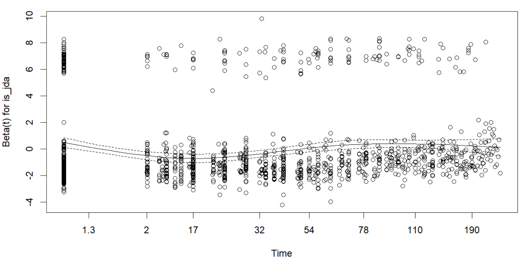
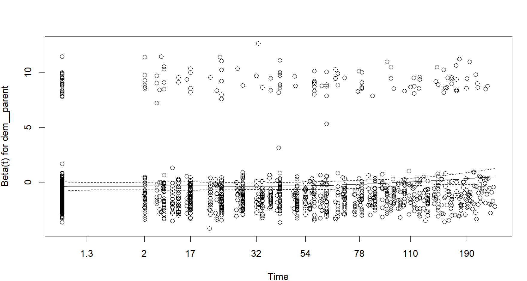
Edit: added new plots generated with plot.cox.zph(), to replace those I had generated with survminer::ggcoxzph(), due to an error in the code of the latter as pointed out by EdM in a comment.

Recently I've been learning about Survival Analysis, and today I'm practicing checking the proportional hazards assumption of a Cox PH regression.

I've read that plotting the Schoenfeld residuals of a certain predictor is a way of assessing the validity of the proportional hazards assumption for that predictor. As I understand it, if the trend line through those residuals is not flat then it suggests the proportional hazards assumption is not valid for that predictor.

But having just done this for two predictors in my Cox PH regression, I am perplexed by the fact that the covariate with the wigglier trend through its Schoenfeld residuals is associated with a much higher p-value than that of the covariate with the less wiggly trend:

The trend in the upper plot is associated with a p-value of 0.887, while that of the lower plot is 0.076.

My question is: why does the wigglier Schoenfeld residual trend have a much higher associated p-value in this case? I assume my being perplexed by this has to do with some lack of understanding of the concepts at play.

Answer 1

The null hypothesis evaluated by cox.zph() is whether the slope of the scaled Schoenfeld residuals versus (transformed) time equals 0. A wiggly curve without an overall trend is hard to distinguish from a straight flat line on that basis, so the result is a very high probability (p-value) that your data for the upper, wiggly curve are consistent with that null hypothesis.

The second curve has a fairly consistent upward trend with time. That makes it much less likely that the null hypothesis of slope = 0 is true. The p-value is "close to significant" by the usual, arbitrary, p < 0.05 criterion.

That said, you might still want to re-evaluate how you model both predictors.

In the top plot it looks like there is a noticeable drop in the coefficient estimate right after the very first time (time = 1?), perhaps from positive to negative, a rise thereafter until about time = 60, and fairly flat thereafter. Does that make sense, based on your understanding of the subject matter? Modeling that predictor with a time-varying coefficient could be considered. See the time-dependence vignette of the R survival package.

Similarly for the second predictor. The p-value isn't technically "significant", but there is a hint of a trend. Is that trend important enough to matter in practice, such that you might need to consider a time-varying coefficient for that as well? There are no cut-and-dried answers to that question; you have to apply your understanding of the subject matter and be able to defend your choice to skeptical reviewers of your work.