Interpreting logistic modelling and linear modelling results for the same formula

Question

I am currently learning how to do statistical modelling in R and realised that if the response variable is dichotomous, it is better to go for logistic modelling as compared to linear modelling.

I used the run17 dataset from the cherryblossom package in R. The run17 dataset contains details for all 19,961 runners in the 2017 Cherry Blossom Run, which is an annual road race that takes place in Washington, DC. The dataset has an event column which denotes whether the participant ran in the "10 Mile" event or the "5 Km" event. I was interested to see if participants' event choice selection was affected by their age and sex. Since the event variable is dichotomous, I first converted it to boolean values (1 = 10 Mile event and 0 = 5 Km event) for it to work with the formula.

As the response variable is dichotomous, I used logistic modelling. But at the same, I also tried linear modelling to see what is difference between them. Given below is the code I used.

# Loading the required packages
if (!require(cherryblossom)) install.packages('cherryblossom')
library(cherryblossom)
library(dplyr)

# Converting event variable values into boolean 
run17_boolean <- run17
run17_boolean$event <- recode(run17_boolean$event, "10 Mile" = 1, "5K" = 0)

# Building the linear model
model_lm <- lm(event ~ sex + age, data = run17_boolean)

# Building the logistic model
model_glm <- glm(event ~ sex + age, data = run17_boolean, family = "binomial")

# Summary of the model
summary(model_lm)
summary(model_glm)

I find that the summary of the models is almost the same. I am still learning how to interpret the model summaries so I may be wrong here. I then tried to plot the model using ggplot2 to see if they are visually similar.

library(ggplot2)

# Linear model
run17_boolean %>% ggplot(aes(age, event, col = sex)) +
  stat_smooth(method = "lm") +
  labs(x = "Age",
       y = "Event",
       title = "Event ~ Age + Sex (linear model)") + 
  theme_bw()

# Logistic model
run17_boolean %>% ggplot(aes(age, event, col = sex)) +
  stat_smooth(method = "glm", method.args = list(family = "binomial")) +
  labs(x = "Age",
       y = "Event",
       title = "Event ~ Age + Sex (logistic model)") + 
  theme_bw()

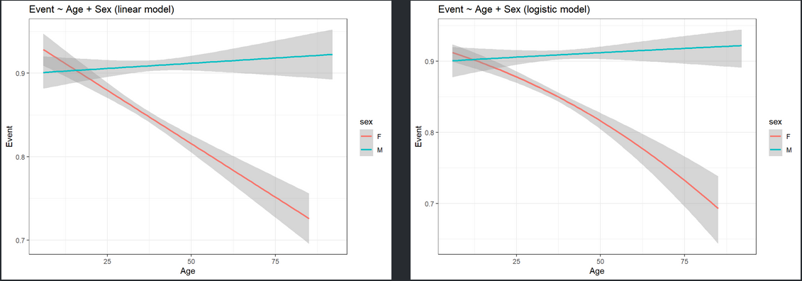
The graphs are also very similar as the fitted values are very similar between the plots.

1. My question is why when linear modelling, which works best for continuous data gave very close results to logistic modelling even when I had a dichotomous response variable?

2. Or is it just a chance that I got very similar results when lm() and glm() was used for this particular data and would not work for other datasets?

Answer 1

why when linear modelling, which works best for continuous data gave very close results to logistic modelling even when I had a dichotomous response variable?

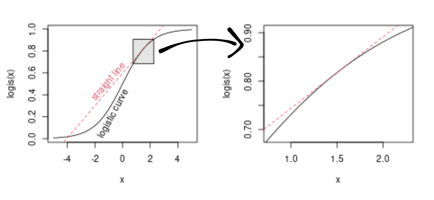
The logistic curve can be approximated with a linear function for a small range. See in the image below a plot of the logistic curve and how in a small range (in the shaded area) the logistic curve is approximately linear.

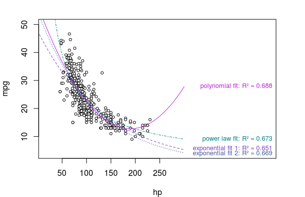
The effect is true for any non-linear function (not just with logistic curves). When the range is very small, and non-linear functions start to be approximately linear, then many different functions can fit the same data reasonably well.

A similar situation is this question (Coronavirus growth rate and its possibly spurious resemblance to vapor pressure model) where data follows an approximately exponential model in a small range and many different models were found to fit the data well (among them an unreasonable fit with a vapour pressure model that has no physical relation with the mechanics of the original problem).

Or here Why would you perform transformations over polynomial regression?

Answer 2

You have quite a lot of data, and very well-behaved data. In such a case, it does happen that the model fits from an ordinary and a logistic regression are close to each other, especially in the "middle" part of fitted probabilities, as are the p-values for the coefficients.

Note, though, that there are differences. The fitted probability as a function of Age is noticeably curved for sex = F in the logistic model, but linear in the OLS model (not surprising, of course, because of the log link). And the confidence region for sex = M at high Ages exceeds 1 in the OLS, which is of course nonsensical.

The key issue is that nonsensical fits (or predictions, or extrapolations) larger than 1 or smaller than 0 can easily happen in OLS models if you have less well-behaved data, for instance if you have lots of 1s in the dependent variable for certain parameter constellations. This can happen more easily, and be harder to detect, in more complex models with more than two parameters.