This answer will confine itself to mutually exclusive classes. The two being compared partitions U and V are two categorical variables, a category is a class "label". (This answer is based on the description document for my SPSS macro !KO_clasagree found on my web-page in the collection "Compare partitions".)
This answer is about classification comparison indices. See a counterpart Q/A about clustering agreement indices.
Group ("label") match between partitions can generally be not complete and the number of groups in partitions can be not equal. Say, U may consist of groups 1, 2 and 3, and V – of groups 1, 2, 4 and 5. In this instance correspondent groups are two (pairs) – 1 and 2, they exist in both partitions; other groups are noncorrespondent and they cannot be the ground of agreement between U and V, on the contrary – they vote for nonagreement. As usual, however, comparing classifications often utilizes data where U and V are entirely made of mutually correspondent groups.
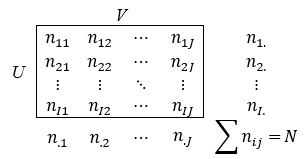
There are two main types of measures: measures for binary classification (these measures’ values can then be averaged into values of multiclass classification) and measures for multiclass classification proper. Both these and those start from the frequency crosstabulation of the being compared partitions U (I groups) и V (J groups) [Fig.1]:

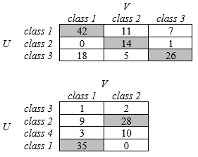
Labels of classes are partly or completely same in U and V. Here are examples of crosstabulations, cells on the crossing of classes of the same label are flagged [Fig.2]:

We’ll designate by letter M the set of classes common in U and V, and by letter K the number of these common classes, 1≤K≤min(I,J). While N is the sum of frequencies of the whole table (= the number of the dataset cases), not only in the K cells flagged in it.
Measures of agreement (similarity) between U and V can be symmetric or asymmetric. A symmetric measure will not change value if U (table rows) and V (table columns) swap their places, i.e., the frequency cross-table get transposed. An asymmetric measure will change value after the table is transposed. For asymmetric measures, it is significant which of the two partitions to consider reference (exemplar, true), and which to consider predicted (experimental). For asymmetric measures, the current answer treats partition U (defining table rows) as the reference classification, and partition V (defining table columns) as the predicted classification $^1$.
Binary classification measures
Measures for binary aka one-hot aka class-specific classification. The focus of interest is a classification in one specific class. Such an agreement measure is calculated for each class k of M. The 2x2 confusion matrix is built, where partition U (rows) is taken for reference classification, and partition V (columns) is taken for predicted classification, if the measure is asymmetric:

This matrix is the IxJ frequency crosstabutation dichotomized. Based on counts a, b, c, d this or that measure is computed. Because there are K such confusion matrices, there are K values of the measure. Below are the formulas of different measures as they are computed for each class-of-interest (positive aka focal class).
Accuracy aka Rand aka Simple Matching coefficient, symmetric, ranges [0,1].
$ACC=(a+d)/N$
1-ACC is called Missclassification (or Error) Rate and is linearly equivalent to the squared euclidean distance.
Recall aka Sensitivity aka True Positive Rate aka Hit Rate aka Positive Accuracy, asymmetric (counterpart value =PRE), ranges [0,1].
$REC=a/(a+b)$
Specificity aka True Negative Rate aka Negative Accuracy, asymmetric (counterpart value =NPV), ranges [0,1].
$SPE=d/(d+c)$
Youden's index, asymmetric, ranges [-1,1].
$YOUD=REC+SPE-1$
Precision aka Positive Predictive Value, asymmetric (counterpart value =REC), ranges [0,1].
$PRE=a/(a+c)$
1-PRE is called False Discovery Rate.
Negative Predictive Value, asymmetric (counterpart value =SPE), ranges [0,1].
$NPV=d/(d+b)$
Markedness index, asymmetric, ranges [-1,1].
$MARK=PRE+NPV-1$
F1 aka F Measure aka Dice Matching coefficient, symmetric, ranges [0,1], it is the harmonic mean of REC and PRE.
$F1=2a/(2a+b+c)=2PRE \cdot REC⁄(PRE+REC)$
F-beta aka generalized or weighted F Measure, generally asymmetric, ranges [0,1], it is the weighted harmonic mean of REC and PRE.
$FBETA=(1+ beta^2)PRE \cdot REC⁄(beta^2 PRE+REC)$
where parameter beta (0,+∞): If beta<1, PRE receives greater weight than REC; if beta>1, REC receives greater weight than PRE. At beta=1 FBETA turns into F1.
Kulczynski 2 coefficient, symmetric, ranges [0,1], it is the arithmetic mean of REC and PRE.
$KULCZ2=(PRE+REC)/2$
logarithm of Diagnostic Odds Ratio, symmetric, ranges [-∞,+∞].
$LNDOR= \ln (ad⁄bc)$
Discriminant Power, symmetric, ranges [-∞,+∞].
$DP= \frac{\sqrt 3}{\pi} (\ln \frac{REC}{1-SPE} + \ln \frac{SPE}{1-REC})$
Matthews correlation aka Phi correlation, symmetric, ranges [-1,1]. This is just the Pearson correlation in case of binary data.
$CORR= \frac{ad-bc}{\sqrt{(a+b)(a+c)(b+d)(c+d)}} = \frac{a/N-SP}{\sqrt{SP(1-S)(1-P)}}$
where $S=(a+b)/N$ and $P=(a+c)/N$.
Balanced Classification Rate, asymmetric, ranges [0,1], it is the arithmetic mean of REC and SPE and it is the AUC (area under the curve) in the ROC space, for a single point there.
$BCR=(REC+SPE)/2$
GM Measure, asymmetric, ranges [0,1], it is the geometric mean of REC and SPE.
$GM=\sqrt{REC \cdot SPE}$
Adjusted GM Measure, asymmetric, ranges [0,1], is a modification of GM designed to better cope with unbalanced classes.
$AGM= \frac{GM+SPE \cdot Q}{1+Q}$, and with $REC=0$, $AGM=0$
where $Q=(d+c)/N$
If the positive class is disproportionally small, this measure may be preferable to GM because it is more sensitive to changes in SPE than to changes in REC.
Optimized Precision, asymmetric, ranges [-∞,1]. The measure is higher when a and d both are high.
$OPRE=ACC - |REC-SPE|/(REC+SPE)$
Jaccard aka Tanimoto Matching coefficient, symmetric, ranges [0,1].
$JACCARD=a/(a+b+c)$
Measures ACC, PRE, NPV, CORR, F1, FBETA, OPRE, JACCARD are sensitive to change in the shape of distribution of objects in classes of reference (U) classification, that is why it is said that these measures are not the same result in situations of balanced and unbalanced classes.
Averaging binary coefficients
A binary coefficient is for one-class-of-interest at a time. If your partitions U and V contain K>2 same-label classes, you may want to obtain one omnibus value as a measure of the multiclass partitions agreement. There can be various approaches how to "combine" or "average" the K values in one, so there may be disagreement among software packages in this respect. [By the way, I would be thankful if readers point me to a discussion in literature on internet about ways to do it.] My macro !KO_clasagree performs arithmetic averaging, optionally weighted:
a. simpe arithmetic mean of the K values
b. weighted arithmetic mean of the K values. Weights are the row marginal frequencies, i.e. the class sizes in partition U. Thus, classes of greater sizes bear more on the averaged result. To Use if the quality of prediction for large classes is more important.
c. like the former, only weights are the inverted row marginal frequencies, therefore classes of smaller sizes bear more on the averaged result. To use if the quality of prediction for small classes is more important.
It is a tricky question "when" the averaging should take place. Should the ready computed coefficients be averaged, or their terms (parts of the formula) should be averaged first and then the coefficient is computed. As for my macro currently, for the following measures, K values get averaged after the measure is computed: ACC, REC, PRE, SPE, NPV, LNDOR, DP, JACCARD. While for the following measures, averaging is done before the measure is computed with its formula: YOUD, MARK, F1, FBETA, KULCZ2, CORR, BCR, GM, AGM, OPRE.
Also to remark: with weighted averaging (b or c) all binary comparison measures become asymmetric, because weights are always the sizes in the reference classification (the one that defines rows of crosstabulation, per my answer).
Multiclass proper aka nominal classification measures
These are symmetric measures of association for two nominal variables, and are known also as measures of experts agreement. Such a measure, its single value, is computed immediately from the complete frequency crosstabulation (see Fig. 1-2 above). The basis of similarity is the frequencies in the cells on the crossings of the same-labelled classes, i.e. the K cells constituting the set M. The measures are similarities.
Overall Success Rate aka Relative Agreement aka Multiclass Accuracy is simply the proportion of correctly (samely) classified objects, the proportion of objects that fall in U and V in groups of the same label.
$OSR= \sum_{i,j∈M}^K n_{ij} ⁄N$
Cohen’s Kappa is OSR normalized by level of random agreement. Ranges in [-∞, 1]. Value 0 means agreement on a random level.
$KAPPA= \frac{P_o-P_e}{1-P_e}$, where observed agreement $P_o=OSR$, and expected random agreement is
$P_e= \sum_{i,j∈M}^K n_{i.} n_{.j} ⁄ N^2$
Scott’s Pi is another way to normalize OSR by level of random agreement. Ranges in [-∞, 1]. Value 0 means agreement on a random level. Formula of SPI is the same as of KAPPA, but
$P_e= \sum_{i,j∈M}^K (n_{i.} + n_{.j})^2 ⁄ (2N)^2$
Brennan–Prediger Kappa – one more way to normalize OSR by level of random agreement, without assuming fixed class sizes (i.e. of marginal frequencies). Ranges in [-∞, 1]. Value 0 means agreement on a random level. Formula of BPK is the same as of KAPPA, but
$P_e= K⁄(IJ)$
If I=J=K, then $P_e= 1/K$ and BPK is linearly equivalent to OSR.
Multiclass Matthews correlation aka Rk correlation. It is Pearson correlation computed bijectively between two sets of dummy variables, ranges in [-1, 1]. If to turn two categorical variables consisting of the same K categories into two sets of binary dummy variables, K columns each, where the columns – they represent the categories – are co-ordered between the sets, then after centering all the columns one should vectorize each NxK set into the column of length NK. Then Pearson r computed by the “cosine formula” between the two obtained columns X and Y is RKCORR:
$RKCORR= \frac{SCP_{xy}}{\sqrt{SS_xSS_y}}$ , where $SCP_{xy}$ is the sum of cross-products of X and Y, and $SS_x$ and $SS_y$ are the sums of squares in the two columns.
Equivalent formula to compute RKCORR from the square KxK crosstabulation with the same, co-ordered categories:
$RKCORR= \frac {\sum_{k,l,m}^K (n_{kk}n_{lm} - n_{kl}n_{mk})} {\sqrt{\sum_k^K (n_{k.} (N-n_{k.})) \sum_k^K (n_{.k} (N-n_{.k}))}}$
RKCORR is computed only if partitions U and V consist of completely the same sets of group labels.
Literature:
- Tharwat, A. Classification assessment methods // Applied Computing and Informatics (2018), https://doi.org/10.1016/j.aci.2018.08.003.
- Labatut, V., Cherifi, H. Evaluation of performance measures for classifiers comparison // Ubiquitous Computing and Communication Journal, 2011, 6, 21-34.
- Hossin, M., Sulaiman, M. A review on evaluation metrics for data classification evaluations // International Journal of Data Mining & Knowledge Management Process (IJDKP), 2015, 5(2), 1-11.
- Sokolova, M., Lapalme, G. A systematic analysis of performance measures for classification tasks // Information Processing and Management, 2009, 45, 427–437.
- Matthews, B.W. Comparison of the predicted and observed secondary structure of T4 phage lysozyme // Biochimica et Biophysica Acta (BBA) - Protein Structure, 1975, 405(2), 442–451.
- Gorodkin, J. Comparing two K-category assignments by a K-category correlation coefficient // Computational Biology and Chemistry, 2004, 28, 367-374.
- Jurman, G., Riccadonna, S,, Furlanello, C. A comparison of MCC and CEN error measures in multi-class prediction // PLoS ONE, 2012, 7(8): e41882, doi:10.1371/journal.pone.0041882.
- Brennan, R., Prediger, D. Coefficient Kappa: some uses, misuses and alternatives // Educational and Psychological Measurement, 1981, 41, 687-699.
- Maxwell, A.E. Coefficients of agreement between observers and their interpretation // Brit. J. Psychiatry, 1977, 530, 79-83.
- Batuwita, R., Palade, V. Adjusted geometric-mean: a novel performance measure for imbalanced bioinformatics datasets learning // Journal of Bioinformatics and Computational Biology, 2012, 10(4), 1250003-1 – 1250003-23.
$^1$ A decision schema around the issue of asymmetric agreement indices. Indices can be symmetric or asymmetric mathematically and partitions can be symmetric or asymmetric positionally. Positionally symmetric partitions is when we're just comparing two alternative partitions. Positionally asymmetric partitions is when one of the two is "reference" and the other is "experimental" - different roles. Then...
If the index is symmetric and the roles are symmetric, then no problem. If the index is symmetric and the roles are asymmetric, we say: the given symmetric index serves the asymmetric roles (like, say, correlation coefficient is still a valid index in a cause-response relationship).
If the index is asymmetric and the roles are symmetric, then, in case of comparison of clustering partitions (i.e., no knowledge of labels is used) we treat the index asymmetry as a mere inconvenience and average/combine the two values (if the action defensible). But in case of comparison of classification partitions (knowledge of labels is used) we refuse the symmetry of roles and move to the situation where one partition is declared "reference" and the other "experimental".
If the index is asymmetric and the roles are asymmetric, then, in case of comparison of clustering partitions we may accept and interpret both distinct values of the index (plus possibly average/combine them into one). In case of comparison of classification partitions we interpret only one of the two values of the index, based on "who is who" in the partitions pair.


