Why does degrees of freedom = $\frac{\operatorname{Tr}(H'H)^2}{\operatorname{Tr}(H'HH'H)}$?

Question

Wikipedia gives the following expression in "degrees of freedom" section, calling it the "Satterthwaite" approximation:

\begin{equation*} \text{df}\approx \frac{\operatorname{Tr}(H'H)^2}{\operatorname{Tr}(H'HH'H)} \tag{1}\label{1} \end{equation*}

where $H=X(X'X)^{-1}X'$ and $X$ is the data matrix.

How/where is this formula obtained? It's not in the references they cite.

---

A slightly more general definition of $H$ which may have originated this formula, is the non-parametric extension -- matrix which maps labels to predictions of the fitted model. AKA "the smoother matrix"

$$\hat{y}=Hy$$

Edit, Sep 27

Possibly related: let $x$ be a multivariate Gaussian random variable and we model $\|x\|^2$ as Chi-Squared with $k$ degrees of freedom. What's $k$? Satterthwaite approximation says to use $k=\text{df}$ from Eq \eqref{1} where $H$ consists of many samples of $x$ stacked as rows.

Excerpt from Encyclopedia of Statistical Sciences, Vol 3:

Answer 1

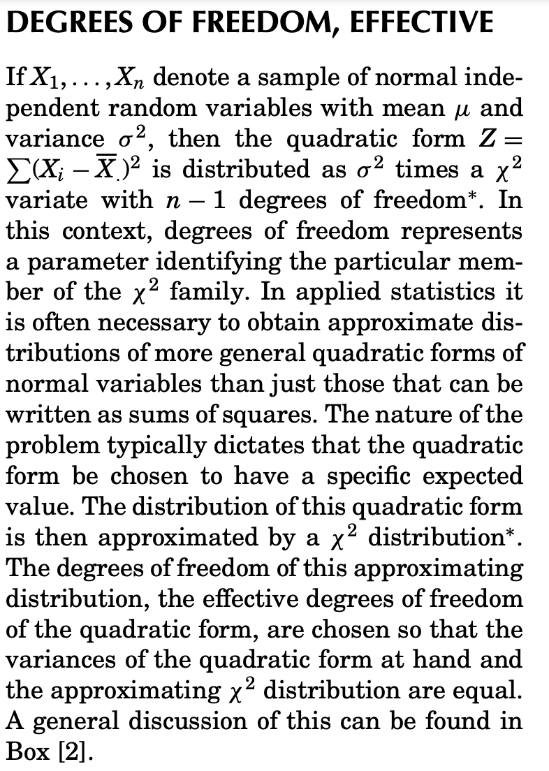
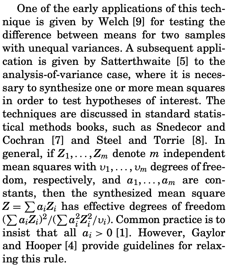
There is a Wikipedia article that is more directly about the Welch-Satterthwaite approximation.

The Wikipedia article makes the following citations to original sources

Satterthwaite, F. E. (1946), "An Approximate Distribution of Estimates of Variance Components.", I Biometrics Bulletin, 2 (6): 110–114

Welch, B. L. (1947), "The generalization of "student's" problem when several different population variances are involved.", Biometrika, 34 (1/2): 28–35

---

The principle behind it is to approximate a sum of squares (as used in several hypothesis tests or estimates of variance), when it is distributed as a linear sum of chi-squared distributions, by a single chi squared distribution.

The approximation applies the methods of moments. For a chi-squared distribution we have that the degrees of freedom is expressed by $k = \frac{\text{Mean}(\chi)^2}{\text{Var}(\chi)}$, and the method of moments uses sample estimates to for the mean and variance.

Let $y_i=\bar{y_i}+\epsilon_i$ be observations of true labels labels $\bar{y_i}$ corrupted with IID zero-centered noise $\epsilon_i$. For a given linear estimator

$\hat{y} = H y$

The sum of squares of the model and the residuals are

$$\begin{array}{rcl} SS_{model} &=& \Vert H (y-\bar{y}) \Vert^2 \\ SS_{residuals} &=& \Vert y- H y \Vert^2 = \Vert (I-H) (y-\bar{y}) \Vert^2 \\ \end{array}$$

If distribution of $y-\bar{y}$ has identity covariance, we have the following expressions for covariance of $\hat{y}$ and $y-\hat{y}$

$$\Sigma_{\hat{y}} = HH^T = H^2$$

$$\Sigma_{y-\hat{y}} = (I-H)(I-H)^T = I - 2H + H^2$$

the distribution of the sum of squares of a multivariate normal distribution can be seen as a sum of the independent principle components with variance equal to the eigenvalues. The sum of these eigenvalues is alse the trace of the covariance matrix.

The mean and variance will be

$$\begin{array}{rcl}\text{mean}(SS_{model}) &= &tr(HH^T) \\ \text{var}(SS_{model})& = &tr((HH^T)^T(HH^T)) = tr((HH^T)(HH^T)) \end{array}$$

and for $SS_{residuals}$ you get something similar but I won't wrote it out as it becomes a bit more complex, but that is where the different expressions come from.

When $H$ is a projection matrix (as in OLS) then $H^tH = H$. That is another source for getting different types of expressions.