What can explain large Odds Ratios 95% confidence intervals in multilevel binomial logistic regression (glmer)?

Question

I conducted a multilevel binomial regression (glmer) and I obtain quite wide confidence intervals for my odds ratio. What could be causing such large 95% CI and what can be done to provide more precise CI? Is it right to assume that odds ratio can be interpreted in the same way for a multilevel logistic regression as for a normal logistic regression?

formal_c <- glmer(formal~type_opld_binary2+gender_binary2+pfeat2+(1 | opleader), data=political_data, family=binomial(link="logit"), control = glmerControl(optimizer = "bobyqa"), nAGQ=1)
summary(formal_c)

ORformal_c <- exp(fixef(formal_c))

CIformal_c<-exp(confint(formal_c, parm= "beta_", method="Wald"))

ORformal_c.CIformal_c <- rbind (cbind(ORformal_c, CIformal_c))
ORformal_c.CIformal_c

I tried a bootstrapping method below but no difference was found...

CIformal_c<-exp(confint.merMod(formal_c, method="boot"))

Here is the output:

Formula: 
formal ~ type_opld_binary2 + gender_binary2 + pfeat2 + (1 | opleader)
   Data: political_data
Control: glmerControl(optimizer = "bobyqa")

     AIC      BIC   logLik deviance df.resid 
   312.0    334.7   -150.0    300.0      322 

Scaled residuals: 
    Min      1Q  Median      3Q     Max 
-3.8863 -0.3788 -0.1705  0.4527  3.4420 

Random effects:
 Groups   Name        Variance Std.Dev.
 opleader (Intercept) 2.865    1.693   
Number of obs: 328, groups:  opleader, 48

Fixed effects:
                            Estimate Std. Error z value Pr(>|z|)
(Intercept)                  0.92427    0.66839   1.383 0.166714
type_opld_binary2athlete    -3.47398    0.93910  -3.699 0.000216
type_opld_binary2influencer -3.67788    0.84842  -4.335 1.46e-05
gender_binary2female         1.50796    0.68908   2.188 0.028642
pfeat2story                  0.09136    0.45331   0.202 0.840274
(Intercept)                    
type_opld_binary2athlete    ***
type_opld_binary2influencer ***
gender_binary2female        *  
pfeat2story                    
---
Signif. codes:  0 ‘***’ 0.001 ‘**’ 0.01 ‘*’ 0.05 ‘.’ 0.1 ‘ ’ 1

Correlation of Fixed Effects:
               (Intr) typ_pld_bnry2t typ_pld_bnry2n gndr_2
typ_pld_bnry2t -0.474                                     
typ_pld_bnry2n -0.480  0.525                              
gndr_bnry2f    -0.398 -0.185         -0.103               
pfeat2story    -0.351  0.036         -0.144         -0.091

                            ORformal_c       2.5 %     97.5 %
(Intercept)                 2.52003814 0.679946015  9.3398477
type_opld_binary2athlete    0.03099351 0.004919372  0.1952683
type_opld_binary2influencer 0.02527639 0.004792244  0.1333187
gender_binary2female        4.51749331 1.170456269 17.4357183
pfeat2story                 1.09566606 0.450625842  2.6640375

I posted this question on stack.overflow and was advised to post it here too (https://stackoverflow.com/questions/74026487/what-can-explain-large-odds-ratios-95-confidence-intervals-in-multilevel-binomi).

Any advice would be appreciated, I'm quite new in those analyses. Thanks!!

Answer 1

This has nothing to do with the multi-level structure of the model (ie. with the random effects). The explanation is that one subgroup (female artistic celebrities) has probability of positive outcome close to 1 (81 "Yes" & 3 "No" vs 14 "Yes" & 17 "No" for male artists). So the corresponding odds ratio is extreme, with a large standard error. It's hard to estimate extreme values precisely.

You have three categorical predictors:

• celebrity: "Artistic", "Sport", "Influencer"
• gender: "Male", "Female"
• post: "Permanent post", " Ephemeral story"

And you fit the generalized linear mixed-effects model (GLMM):

politics ~ celebrity + gender + post + (1 | ID)

Note: I've renamed the variables for readability.

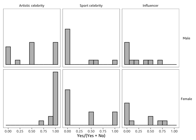
Only the confidence interval for the gender = "Female" odds ratio is wide. To understand what's going on, it really helps to look at the raw data.

Below I compute the observed probability of politics = "Yes" for each celebrity and plot a histogram of the probabilities for each combination of gender and celebrity type. (I ignore whether the post is permanent or ephemeral.)

A couple of observations: There doesn't seem to be much difference between the two genders as far as sports celebrities and influencers are concerned. The "action" is all in the group of artistic celebrities where female celebrities seem to post only about politics. (Strange? You should consider carefully how the celebrities were selected and how their social media posts were collected and labeled. It would be hard to take the data at face value otherwise.)

Note that this suggests that there is an interaction between celebrity type and gender, so I fit this model instead:

politics ~ celebrity * gender + post + (1 | ID)

The GLMM has to model this pattern and so the log odds ratio for female celebrities is large: $\hat{\beta}_{\text{Female}}$ = 4.1. Once you exponentiate to get the odds ratio, its confidence intervals is very wide because the estimate is so extreme. The model has basically concluded that female artistic celebrities have much higher odds to post about politics than male artistic celebrities but it's hard to be precise about how much higher.

#>                                           2.5 %     97.5 %
#> (Intercept)                           -1.542109  1.1936138
#> celebritySport celebrity              -4.050401  0.5909732
#> celebrityInfluencer                   -3.282459  0.6970215
#> genderFemale                           2.106927  6.5826006
#> postEphemeral story                   -1.009981  0.7741624
#> celebritySport celebrity:genderFemale -6.843921 -0.4383856
#> celebrityInfluencer:genderFemale      -8.049952 -1.8693357

I think it's a bit more helpful to look at pairwise comparisons between male and female celebrities (for each celebrity type) rather than the model coefficients. (I use the emmeans package.)

pairs(emmeans(model, ~ gender | celebrity, type = "response"))
#> celebrity = Artistic celebrity:
#>  contrast      odds.ratio     SE df null t.ratio p.value
#>  Male / Female     0.0159 0.0175 67    1  -3.764  0.0004
#> 
#> celebrity = Sport celebrity:
#>  contrast      odds.ratio     SE df null t.ratio p.value
#>  Male / Female     0.5811 0.6698 67    1  -0.471  0.6392
#> 
#> celebrity = Influencer:
#>  contrast      odds.ratio     SE df null t.ratio p.value
#>  Male / Female     1.6930 1.6650 67    1   0.535  0.5942
#> 
#> Results are averaged over the levels of: post 
#> Tests are performed on the log odds ratio scale

---

R code to reproduce the plot and the analysis. I use glmmTMB instead of lme4 to fit the GLMM.

library("glmmTMB")
library("emmeans")
library("tidyverse")

political_data <-
  here::here("591906.sav") %>%
  haven::read_sav() %>%
  mutate(
    across(where(labelled::is.labelled), labelled::to_factor)
  ) %>%
  rename(
    politics = formal,
    celebrity = type_opld_binary2,
    gender = gender_binary2,
    post = pfeat2,
    ID = opleader
  ) %>%
  mutate(
    gender = forcats::fct_rev(gender)
  ) %>%
  select(
    politics, celebrity, gender, post, ID
  )

political_data2 <- political_data %>%
  group_by(
    ID, celebrity, gender, post
  ) %>%
  summarise(
    Yes = sum(politics == "Yes"),
    No = sum(politics == "No")
  )

political_data2 %>%
  group_by(
    post,
    .add = TRUE
  ) %>%
  summarise(
    Yes = sum(Yes),
    No = sum(No)
  ) %>%
  ggplot(
    aes(Yes / (Yes + No))
  ) +
  geom_histogram(
    breaks = seq(-0.05, 1.05, by = 0.1),
    fill = "gray", color = "black"
  ) +
  facet_grid(
    gender ~ celebrity
  ) +
  theme(
    axis.title.y = element_blank(),
    axis.ticks.y = element_blank(),
    axis.text.y = element_blank()
  )

model <- glmmTMB(
  cbind(Yes, No) ~ celebrity * gender + post + (1 | ID),
  family = "binomial",
  data = political_data2
)
confint(
  model,
  "beta_",
  method = "profile"
)

pairs(emmeans(model, ~ gender | celebrity, type = "response"))

Answer 2

There can be a number of reasons for this. Maybe your random effects cluster doesn't have enough groupings so it doesn't provide a very precise teasing apart of the fixed and random effects. Maybe you have not met the linearity assumption of the model or it has a fairly odd distribution, causing the predictiveness of the predictor to be fairly low. Maybe you have the wrong link function or there is some other confounding factor you haven't considered such as another independence of data effect not modeled in your regression. If there are a fairly low number of observations this can also lead to less precision in your CI.

Without knowing much else about the data/model, this is probably the best I can say on what's going on. Otherwise its difficult to say for certain. Check your model to see if it meets the basics for running a GLMM in the first place.