2
$\begingroup$

I runned two GLMs using the same dependent and independent variables, but modelling each analysis according a different type of distribution. Then, I compared its AIC values to find what distribution best fits the data:

> glm_1 <- glm(data$Y ~ data$X, family = "gaussian")

> glm_2 <- glm(data$Y ~ data$X, family = "Gamma")

> AIC(glm_1, glm_2)
       df      AIC
glm_1  3       38.52803
glm_2  3       26.09031

As you can see, the Gamma distribution better explains my data distribution. However, when performing a Shapiro-Wilk test, I got an indication that there is normality in Y:

> shapiro.test(data$Y)

    Shapiro-Wilk normality test

data: data$Y
W = 0.88314, p-value = 0.1417

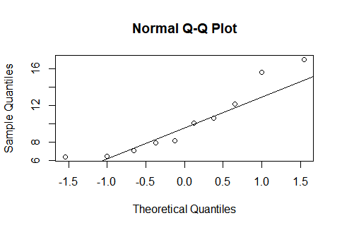
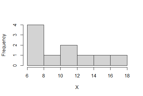
When viewing the distribution of Y on a histogram and on a Q-Q plot, I couldn't convince myself that the distribution is normal:

hist(data$Y, main = " ", xlab = "X")

enter image description here

qqnorm(data$Y)
qqline(data$Y)

enter image description here

According to the results above, would it be incorrect if I performed a simple linear regression of Y ~ X, or would it be more appropriate to make a GLM considering the Gamma distribution?

$\endgroup$
11
  • 3
    $\begingroup$ Hi Filipe! I'm here to share the good news: you don't need to have a normal Y variable! Actually, it's your residuals after fitting the model that need to be normal. $\endgroup$ Commented Oct 16, 2022 at 1:34
  • 1
    $\begingroup$ Do you only have ten points? $\endgroup$
    – Dave
    Commented Oct 16, 2022 at 1:37
  • 2
    $\begingroup$ With ten points, you have basically no power to reject. That is, you claim to have a normal distribution because your hypothesis test for normality fails to reject, but if you did a test for a gamma, I would not expect that to reject, either. $\endgroup$
    – Dave
    Commented Oct 16, 2022 at 2:02
  • 1
    $\begingroup$ @Filipe Failure to reject a null does not mean the null is true. It simply means you can't clearly tell that it's false. Note that if you tested a wide array of other possible distributions, you would fail to reject many of them, but they're mutually exclusive possibilities, they can't all be true (e.g. if I tested goodness of fit for a shifted Weibull, I bet I would not reject that). With 10 data points, won't be able to rule out a wide array of possible distributions. Many posts on site discuss this issue in more detail. $\endgroup$
    – Glen_b
    Commented Oct 16, 2022 at 2:08
  • 1
    $\begingroup$ @Filipe Good points from other commenters about accepting nulls. But we should also point out the robustness of linear regression to the normality assumption, and this, combined with the fact that your data seem pretty "tame" (i.e. no crazy outliers), would lead me to being comfortable fitting a least-squares estimated linear model on your data. $\endgroup$ Commented Oct 16, 2022 at 2:25

1 Answer 1

1
$\begingroup$
  1. Remember that failing to reject the null hypothesis is NOT accepting the null hypothesis. The Shapiro-Wilk test is a test of the null hypothesis of normality. The power of a test is in part a function of sample size. Therefore, if you have few observations, you're unlikely to be able to reject the null (although there are some caveats to this I won't go into) as the test is not well-powered to detect small departures from normality. The main takeaway being the test is not very useful when you have very little data.

  2. However, the test is ALSO not very useful when you have lots of data! Imagine you have infinite data but you distribution is only a tiny bit different from what you'd expect of a normal distribution. The test will give you a p-value pretty much at 0 indicating non-normality. But of course, that's not very useful -- your test told you it's not normal, but what you really care about is just how not normal is it. The test won't get you there. This is a general feature of "testing" assumptions using point nulls.

  3. You seem to think the data being normal is the Gauss-Markov assumption. That is decidedly not the case! See the first two paragraphs: https://en.wikipedia.org/wiki/Gauss%E2%80%93Markov_theorem

  4. Even if it was, the assumption is not about the data -- it's about the error term. Note that the error term is NOT the model residual. The error term is something you do not observe. The residual is specific to your model.

  5. The Gamma distribution might better fit your data, but model fit statistics can be not-so-great. Ideally you'd be able to test on out-of-sample prediction with some more data not used to train your model.

  6. More generally, the Gamma distribution is bounded from below by 0: i.e. it only has support on $(0,\inf)$. If you data can EVER be negative, then it would be quite silly to use that likelihood since you would be using a model that cannot possibly produce the population data, even if it fits your sample well enough.

$\endgroup$
5
  • $\begingroup$ Thank you very much for the detailed answer, everything you and the other commenters explained made me think profoundly about my data! I would just like to clarify a few points: How could I, in R, visualize the error terms? Or, in case I really can't observe this, would the residuals of the model be enough to answer whether it would be ideal to use a simple linear regression? $\endgroup$
    – user351644
    Commented Oct 16, 2022 at 20:18
  • $\begingroup$ You can't observe it. The way to think about this is that the "true" process generating your outcome Y might be Y = bX + e where b is some coefficient for your data X and e is the error term usually assumed normally distributed with fixed variance and mean 0. The error term is just variation in y not explained by x. However, when you run your regression you get an equation y* = bx + e where * indicates it is estimated. The idea is that your don't know FOR SURE that the b* you estimate is the true b (thus p-values etc.). Accordingly, e* ("the model residual") is not always e (the error). $\endgroup$ Commented Oct 16, 2022 at 23:27
  • $\begingroup$ Any time you fit a linear regression with OLS or whatever, you are FORCING the residuals to be drawn from a normal distribution. In reality, the underlying true "errors" might not be normally distributed! Imagine for example you use OLS with a binary outcome - the errors cant be normal but the model will assume they are. If you have few observations, you might at first tbink "oh the errors are normal i just dont have a lot of data to show it" but actually more data would show weird patterns of your errors in relation to the data (e.g. heteroskedasticity) Long ramble on my phone but tldr u cant $\endgroup$ Commented Oct 16, 2022 at 23:33
  • $\begingroup$ Finally, you CAN look at your residuals. They are useful because they can help you diagnose if the normality assumption is not very good, but you can never be certain the underlying errors are non-normal. In R, you can extract residuals from the model fit object and plot them against variables as you please to e.g. assess heteroskedasticity. Q-Q plots are often used for this. A quick Google should get you what you want. $\endgroup$ Commented Oct 16, 2022 at 23:40
  • $\begingroup$ AND FINALLY, giving a plot of the distribution of your actual outcome (the raw data, not a smoothed density estimate or histogram) can help people figure out what likelihood would be appropriate (i.e. what assumptions you want to make about the errors). You can also use robust standard errors to not really worry about your standard errors (the coefficients themselves won't change) if you have a decent sample size. It will be less efficient in most cases, but avoids risk of inconsistency of your variance estimates (p-values, SEs etc.). $\endgroup$ Commented Oct 16, 2022 at 23:43

Your Answer

By clicking “Post Your Answer”, you agree to our terms of service and acknowledge you have read our privacy policy.