What is the difference between CUPED and regression adjustment？

Question

CUPED (Controlled-experiment Using Pre-Existing Data) is a variance reduction technique created by Microsoft in 2013 and widely used in technology companies. let Y is the target metrics and X is pretreatment covariate, T is treat variable(to simplify the discussion, we assume that there are only two treatment group, T = 0 is control group, T = 1 is treat group)，the main idea of CUPED is:

• compute $\theta$

$$\theta = \frac{\operatorname{cov}(Y, X)}{\operatorname{var}(X)} = \operatorname{corr}(X, Y) \cdot \operatorname{var}(Y) = \rho \cdot \operatorname{var}(Y)$$

• compute adjusted $Y_i^{cv} = Y_i - (X_i - \mu_X) \cdot \theta$ for each user

• evaluate the AB test using $Y_i^{cv}$ instead of $Y_i$

the result cuped-adjusted estimate treat effect is

$$\tau = (\overline Y_1 - \theta \cdot (\overline X_1 - \mu_X)) - (\overline Y_0 - \theta \cdot (\overline X_0 - \mu_X)) \\= (\overline Y_1 - \overline Y_0) - \theta \cdot (\overline X_1 - \overline X_0)$$

Another widely used and long-established method for increase power and adjusting preexisting differences is ANCOVA(Analysis of covariance) or regression-adjustment.

The ANCOVA model assumes a linear relationship between the response (Y) and covariate (X):

$$ Y = b_0 + \tau \cdot T + \theta\cdot X $$

the result regression-adjusted estimate treat effect is same as above, the only difference seems to be how to estimate $\theta$, so My questions is which one is more reasonable ?

Answer 1

There is no difference.

First, note that the estimator $\theta$ you describe in CUPED is identical to the slope estimate from simple linear regression.

Second, note that $Y_i^{cv}$ looks curiously like a residual. In that case $Y_i$ would be the dependent variable and $X_i - \mu_x$ would be the regressor.

Third, note that the evaluation of the AB test is done on these residuals (i.e. on $Y_i^{cv}$ as opposed to $Y_i$). Since treatment is often randomly assigned, it is uncorrelated with any other regressors. Hence, the regression coefficient for treatment (and for $Y_{i}$) should be the same if we include treatment in the regression or not. Ostensibly, we could:

• First regress experiment outcomes on pre experiment data. then
• Take the residuals from that regression, and
• Fit another simple linear regression of treatment status onto the residuals

This intuition is formalized by the Frisch–Waugh–Lovell theorem.

From these three pieces alone, it is convincing to see CUPED as a form of regression adjustment. I will leave more formal proof to someone else, but perhaps some simulation would be sufficient icing on the cake.

I will simulate correlated outcomes and artificially inflate the expectation of the second outcome based on random assignment to exposure. I'll then compute the treatment effect via OLS and CUPED. We'll see that the resulting estimates are very similar.

set.seed(0)

N <- 10000
trt <- rbinom(N, 1, 0.5)
Sigma <- matrix(c(1, 0.8, 0.8, 1), nrow = 2)
Y <- MASS::mvrnorm(N, c(0, 0), Sigma)
Y[, 2] <- 0.5*trt + Y[, 2]


# Linear model

fit <- lm(Y[, 2] ~ Y[, 1] + trt)


# CUPED
theta <- cov(Y[, 1], Y[, 2]) / var(Y[, 1])
y_cv <- Y[, 2] - (Y[, 1] - mean(Y[, 1]))*theta
fit_cuped <- lm(y_cv ~ trt)

coef(fit_cuped)['trt']
#>       trt 
#> 0.4976049
coef(fit)['trt']
#>       trt 
#> 0.4976445

^{Created on 2023-12-05 with reprex v2.0.2}

Answer 2

For variance-reduction of randomized experiments/AB tests, ancova/regression-adjust is a more appropriate method to estimate $\theta$, because it takes into account the differences in pre-treat variables between treat/control group before experiment, and the treatment effect during experiment.

sim

cuped

Some simulation data are generated below:

library(tidyverse)
library(mvtnorm)

N <- 10000 # sample size
tau <- 1.2 # treat effect, to make the problem clearer, we assume a relatively large value
cor_mat <- matrix(c(1.0, 0.6, 0.6, 1.0), 2, 2) # assuming a moderately correlation between x and y
cor_mat

     [,1] [,2]
[1,]  1.0  0.6
[2,]  0.6  1.0

xy <- mvtnorm::rmvnorm(N, c(0.0, 0.0), cor_mat) 
df <- tibble::tibble(
  x = xy[, 1],
  t = sample(0:1, N, TRUE),
  y = xy[, 2] + t * tau
)

cuped suggests to estimate $\theta$ by from the pooled population of control and treatment. The way to manually calculate $\theta$ is as follows:

df %>%
  mutate(
    myg = mean(y), # global mean y
    mxg = mean(x), # global mean x
  ) %>%
  summarise(
    vary = sum((y - myg) ^ 2),
    varx = sum((x - mxg) ^ 2),
    covxy = sum((x - mxg) * (y - myg)),
    r = covxy / sqrt(vary * varx),
    b = covxy / varx
  )

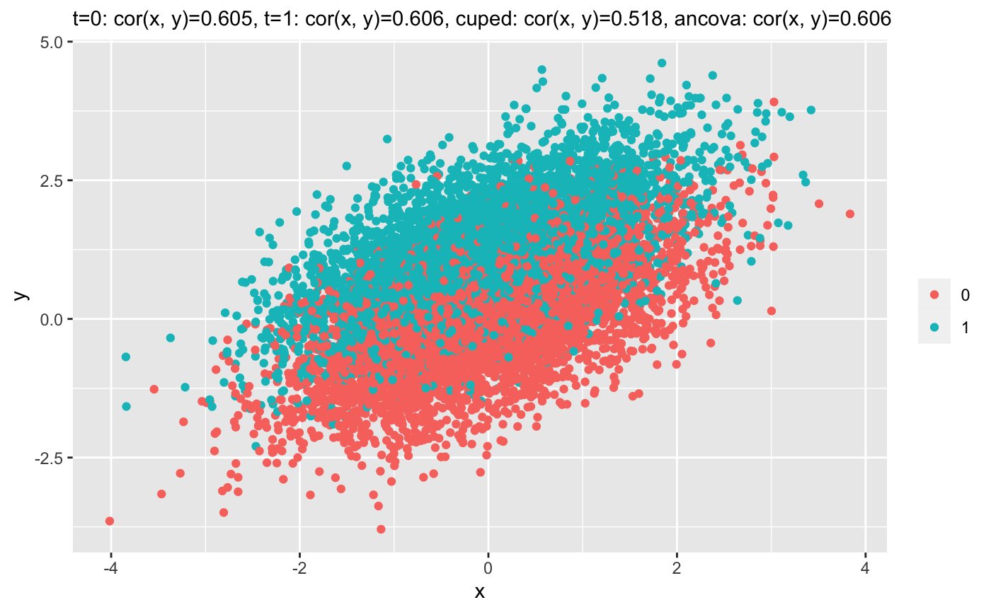
the estimated correlation coefficient(r = 0.518) is smaller than the specified value (r = 0.6) due to simply pool strategy.

ancova/regression-adjust

ancova compute the y and x correlation separately for each group and find the pooled within-group correlation. This is also exactly the coefficient of the covariate estimated by ols

df %>%
  group_by(t) %>%
  mutate(
    myg = mean(y), # mean y for each group
    mxg = mean(x), # mean x for each group
  ) %>%
  ungroup() %>%
  summarise(
    vary = sum((y - myg) ^ 2),
    varx = sum((x - mxg) ^ 2),
    covxy = sum((x - mxg) * (y - myg)),
    r = covxy / sqrt(vary * varx),
    b = covxy / varx ## same as lm(y ~ t + x, df)$coef['x']
  )

the estimated correlation coefficient(r = 0.606) is close to the specified value (r = 0.6) .