Linear mixed effect model, repeated measures or non-parametric test?

Question

I have this study design: two groups (A & B) measured in 3-time points (pre, follow-up & post). I thought that a linear mixed model effect was the preferred option because I do have missing values at random instead of using repeated measures ANOVA. Here is an example of my model:

m0<-lmer(VD ~ Group*Time + (1|ID))#linear model DV predicted by the IV (Group*time)
summary(m0)
anova(m0)#show model as anova
eta_sq(m0, partial=TRUE) #partial eta sq
r.squaredGLMM(m0)#adjust R2 for the model as an alternative

emmeans(m0, pairwise~Group)
emmeans(m0, pairwise~Time, adjust="bonferroni")
emmeans(m0, pairwise~Time|Group)

qqnorm(resid(m0))

Here's the output:

Type III Analysis of Variance Table with Satterthwaite's method
            Sum Sq Mean Sq NumDF  DenDF F value    Pr(>F)    
Group          4.6     4.6     1 185.50  0.0049 0.9442174    
Time       12756.9 12756.9     1 144.14 13.7144 0.0003024 ***
Group:Time   946.4   946.4     1 143.14  1.0175 0.3148195    
---
Signif. codes:  0 ‘***’ 0.001 ‘**’ 0.01 ‘*’ 0.05 ‘.’ 0.1 ‘ ’ 1
> eta_sq(m1, partial=TRUE) #partial eta sq
# Effect Size for ANOVA (Type III)

Parameter  | Eta2 (partial) |       95% CI
------------------------------------------
Group      |       2.65e-05 | [0.00, 1.00]
Time       |           0.09 | [0.03, 1.00]
Group:Time |       7.06e-03 | [0.00, 1.00]

r.squaredGLMM(m1)#adjust R2 for the model as an alternative
            R2m       R2c
[1,] 0.07850414 0.2317482
> 
> emmeans(m1, pairwise~Group)
NOTE: Results may be misleading due to involvement in interactions
$emmeans
 Group emmean   SE   df lower.CL upper.CL
     0   43.3 3.71 74.3     36.0     50.7
     1   37.7 3.72 75.7     30.3     45.1

Degrees-of-freedom method: kenward-roger 
Confidence level used: 0.95 

$contrasts
 contrast        estimate   SE df t.ratio p.value
 Group0 - Group1      5.6 5.25 75   1.066  0.2897

Degrees-of-freedom method: kenward-roger 

> emmeans(m1, pairwise~Time)
NOTE: Results may be misleading due to involvement in interactions
$emmeans
  Time emmean   SE df lower.CL upper.CL
 0.957   40.5 2.63 75     35.3     45.8

Results are averaged over the levels of: Group 
Degrees-of-freedom method: kenward-roger 
Confidence level used: 0.95 

$contrasts
 contrast  estimate SE df z.ratio p.value
 (nothing)   nonEst NA NA      NA      NA

Results are averaged over the levels of: Group 
Degrees-of-freedom method: kenward-roger 

> emmeans(m1, pairwise~Time|Group)
$emmeans
Group = 0:
  Time emmean   SE   df lower.CL upper.CL
 0.957   43.3 3.71 74.3     36.0     50.7

Group = 1:
  Time emmean   SE   df lower.CL upper.CL
 0.957   37.7 3.72 75.7     30.3     45.1

Degrees-of-freedom method: kenward-roger 
Confidence level used: 0.95 

$contrasts
Group = 0:
 contrast  estimate SE df z.ratio p.value
 (nothing)   nonEst NA NA      NA      NA

Group = 1:
 contrast  estimate SE df z.ratio p.value
 (nothing)   nonEst NA NA      NA      NA

Degrees-of-freedom method: kenward-roger 

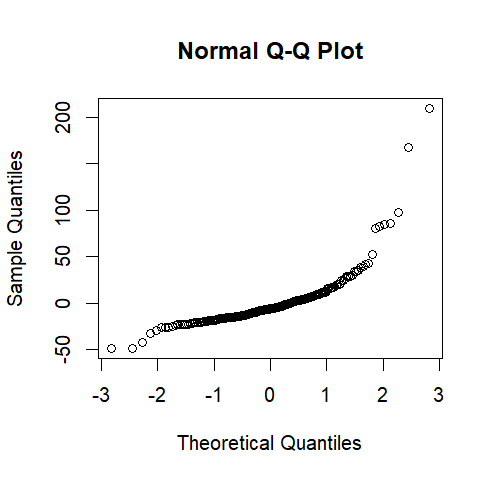
However, when plotting the residuals it does not follow a normal distribution. It doesn't happen to all variables, only a few. Therefore, I was wondering whether I could still use mixed-effect models or if I should still move to a non-parametric test (if yes, which one would be best for my study design) or maybe try to log transform the variables.

Answer 1

You have a modeling problem, as well as possibly a non-normality problem. My reading is that you have three time points, but if you look at the anova, you have 1 d.f. for Time because it is being modeled as a quantitative predictor rather than a factor. That's why in your emmeans output, you have results for just one time value -- the average value of Time -- rather than the three time points, and no comparisons for time.

So the non-normality is the lesser of your problems, given that the model itself has no reasonable interpretation.

For starters, I suggest fitting models like this:

m1 <- lmer(DV ~ Group * factor(Time) + (1|ID), data = data)

I suspect you may still have a non-normality problem for some response variables. That often comes up because the variation in the data is related to the mean, and you can tell the most about that situation by plotting the residuals vs. the fitted values:

plot (resid(m1) ~ predict(m1))

There will be six stacks of points for this model. If those vary in scatter is a systematic way (especially if they get more dispersed to the right than to the left), it can often be helped by transforming the response variable, e.g.,

m2 <- lmer(sqrt(DV) ~ Group * factor(Time) + (1|ID), data = data)
    ### or ###
m3 <- lmer(log(DV) ~ Group * factor(Time) + (1|ID), data = data)

The EMMs will then be on the transformed scale, but you can put the means (not the comparisons) back on the response scale by adding type = "response" to the emmeans() call.

It may serve you well to find a statistical consultant. It is vitally important to get the model right and to understand what you have. It isn't enough to just be able to get programs to run.