When will L2 norm and squared L2 norm be equivalent in ridge regression?

Question

I am doing ridge regression and am wondering why it uses squared L2 norm. This post Why l2 norm squared but l1 norm not squared? gave some thought about why using it. But a further question arises: when will using L2 and squared L2 norm be equivalent?

In my case, I am dealing with a completely orthonormal case. It is a cell-means model with the objective function in the form $\sum_i\sum_j(X_{ij}-\mu_i)^2$:

• Using squared L2 norm adds a term $\lambda(\mu_1^2+\cdots+\mu_p^2) $ to the objective function, which then reduces to p separate univariate optimizations.
• Using L2 norm adds a term $\lambda\sqrt{(\mu_1^2+\cdots+\mu_p^2)} $, which cannot be reduced to univariate optimizations because of the square root of sum of all parameters.

In this case, I don't think those two are still equivalent. So which one to use?

(I think from the KKT condition we should conclude that those two are equivalent, so is there something in the orthonormal case that violates some assumptions?)

Answer 1

Example with 2-fold cross validation

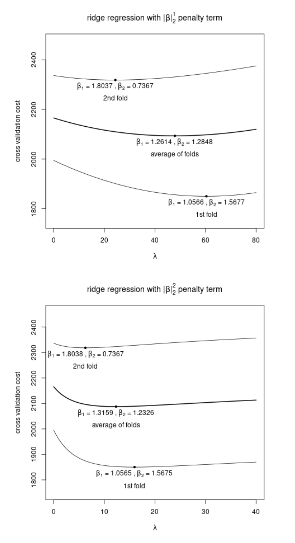
Below is a plot for an example of ridge regression (with the different expressions of the penalty) and 2-fold cross validation for a model

$$y = \beta_1 x_1 + \beta_2 x_2 + \text{noise}$$

The plot shows the cost (sum of squared residuals) in the validation data when the model is fitted with different penalty parameters $\lambda$. The plot has three curves. Two times a thin curve for the single folds, and one time a thick curve for the average of the two folds.

When we choose the $\lambda$ based on the lowest cost in the cross validation data, then the values of the coefficients $\beta$ will be the same (up to some small computational errors) if we do this with a single fold/dataset. But the values will be different when we do this with the average of multiple datasets.

Figure below: the coefficients $\beta$ are the same with cross validation using a single fold, but not when combining multiple folds

What is going on in the above example?

The different norms relate to the same optimisation problem, where we minimize the sum of squared residuals (least squares regression), conditional to the vector of coefficients $\vec\beta$ being inside a sphere of a certain size. Whether we choose/express the sphere as $\Vert \vec\beta \Vert_2^2 \leq t^2$ or $\Vert \vec\beta \Vert_2 \leq t$, is the same.

For every $\lambda_a$ with the one norm there is a different $\lambda_b$ that gives the same solution with the other norm. (The $\lambda_a$ and $\lambda_b$ that give the same solution $\vec{\beta}$ will differ by a factor $2\Vert \vec{\beta} \Vert_2$, more about that further below)

However, the relationship between $t$ and the $\lambda$'s will be different for different data. So the equivalence does not occur when you apply ridge regression to multiple different datasets (eg when we perform n-fold cross validation which uses an average of multiple data subsets).

Single dataset

When we perform cross validation with only a single training dataset then we get a range of solutions $\vec{\beta}$ that will be the same for both norms (only obtained with different values of $\lambda$). We pick the $\vec{\beta}$ that optimizes some cost function in the validation data set and that will be the same for both norms. We see this in the image above. The minima of the cost with single folds are associated give the same $\beta$ values (and the minima occur for different $\lambda$).

In this case the two different norms will give the same fit.

Multiple datasets

However, a breakup of the equivalence occurs when we perform fitting with multiple training data sets (and compute some optimal average).

The comparison that is often made is an average of the performance with several training data folds (the average computed while keeping $\lambda$ the same with each fold).

In this case the two different norms will not give (exactly) the same fit.

Approximately the same with multiple datasets

The different types of regression will be still the same for different datasets when we tune $t$ instead of $\lambda$ (which is not what is done), or when the norm of the solution $\vec\beta$ is the same (in that case you get the same relationship between $t$ and $\lambda$ for the different sets of data).

In practice the norm of $\beta$ for different data sets will not be much different (different training folds will relate to about the same pattern) and you get practically the same results for the two different norms.

Relationships between the two norms

which cannot be reduced to univariate optimizations because of the square root of sum of all parameters.

The gradients of the two are very similar

$$\nabla (\beta_1^2+\dots+\beta_p^2) = 2 \begin{bmatrix} \beta_1 \\ \vdots \\ \beta_p \end{bmatrix}$$

$$\nabla \sqrt{(\beta_1^2+\dots+\beta_p^2)} = \frac{1}{\sqrt{(\beta_1^2+\dots+\beta_p^2)}} \begin{bmatrix} \beta_1 \\ \vdots \\ \beta_p \end{bmatrix}$$

and they only differ in magnitude, but not in direction.

So if $\vec{\beta}$ is a solution with the squared L2 norm and penalty parameter $\lambda_a$, then $\vec{\beta}$ is a solution with the L2 norm and penalty parameter $\lambda_b = \lambda_a 2 \Vert \vec{\beta} \Vert_2 $

Demonstration with code

set.seed(1)
n = 50
control = list(reltol = 10^-18) ### for improving numeric precision of optim optimization

### data
x = rnorm(n)
y = rnorm(n)
z = 2*x + 2*y + rnorm(n, 0, 10)

### selection for splitting data into two folds/subsets
### we use notations [-sel] and [sel] to choose the different folds
sel = sample(1:n,n/2)


### cost function for ridge regression
### with the variable power we can change the expression of the penalty term
### with power = 2 we could also compute more directly using the matrix solution

f = function(par, x, y, z, lambda = 1, power = 2) {

  ### parameters and fit of z  
  a = par[1]
  b = par[2]
  zfit = a*x+b*y

  ### compute cost function
  rss = sum((zfit-z)^2)
  penalty = lambda*(a^2+b^2)^(power/2)

  ### return the result
  return(rss+penalty)
}


### perform the code below with L2 and L2 squared
### by selecting power = 1 and power = 2
for (power in 1:2) {

  ### range of lambda values
  ### and variables to store the cost values and fitted beta 
  ls = seq(0,80,0.01)/power
  cost1 = c()
  cost2 = c()
  beta1 = c()
  beta2 = c() ### these four vectors are empty and will be filled during the for-loop below

  ### perform ridge with different lambda ls
  ### the procedure is done twice (2-fold cross validation)
  for (k in 1:length(ls)) {
    ### perform ridge regression 
    fit = optim(c(2,2), f, 
                x = x[sel], y =  y[sel], z = z[sel], 
                lambda = ls[k], power = power, 
                control = control)
    ### compute cost for cross validation data
    cv_z = fit$par[1] * x[-sel] + fit$par[2] * y[-sel]
    cost1 = c(cost1,sum((cv_z-z[-sel])^2))
    beta1 = cbind(beta1, fit$par)

    fit = optim(c(2,2), f, 
                x = x[-sel], y =  y[-sel], z = z[-sel], 
                lambda = ls[k], power = power, 
                control = control)
    ### compute cost for cross validation data
    cv_z = fit$par[1] * x[sel] + fit$par[2] * y[sel]
    cost2 = c(cost2, sum((cv_z-z[sel])^2))
    beta2 = cbind(beta2, fit$par)
  }

  ### average of two folds
  costm = (cost1+cost2)/2
  betam = (beta1+beta2)/2

  ### plotting
  plot(ls, cost1, type="l", ylim = range(c(cost1, cost2))+c(-100,100), xlab = 
  expression(lambda), ylab = "cross validation cost")
  lines(ls, cost2)
  lines(ls, costm, lwd = 2)

  title(bquote("ridge regression with "*"|"*beta*"|"[2]^.(power)* " penalty term"))

  ### compute the solutions of the beta at the minima
  k1 = which.min(cost1)
  k2 = which.min(cost2)
  km = which.min(costm)

  ### add points in the graph
  points(ls[k1],cost1[k1], pch = 20)
  points(ls[k2],cost2[k2], pch = 20)
  points(ls[km],costm[km], pch = 20)

  text(ls[k1],cost1[k1] - 50, "1st fold", pos = 1)
  text(ls[k1],cost1[k1],
       bquote(beta[1] *" = "* .(round(beta1[1,k1],4)) * " , " * beta[2] *" = "* .(round(beta1[2,k1],4)) ),
       pos = 1)
  text(ls[k2],cost2[k2] - 50, "2nd fold", pos = 1)
  text(ls[k2],cost2[k2],
       bquote(beta[1] *" = "* .(round(beta2[1,k2],4)) * " , " * beta[2] *" = "* .(round(beta2[2,k2],4)) ),
       pos = 1)
  text(ls[km],costm[km] - 50, "average of folds", pos = 1)
  text(ls[km],costm[km],
       bquote(beta[1] *" = "* .(round(betam[1,km],4)) * " , " * beta[2] *" = "* .(round(betam[2,km],4)) ),
       pos = 1)

}

Answer 2

The definition of ridge regression uses the squared $L2$ norm for the penalty. The objective function is

$$L(\beta; \lambda) = \sum_{i = 1}^{n}(y_i - x_i\beta)^2 + \lambda \sum_{j = 1}^{p} \beta_j^2 \space \space,$$ where $p = \dim(\beta)$. In that sense, your question has an easy answer: Ridge regression uses the squared $L2$ norm because that's the defition of ridge regression.

If all you care about is getting the correct coefficients, it doesn't matter if you use the $L2$ norm or its square. Compare the two objective functions term by term:

$$\sum_{i = 1}^{n}(y_i - x_i\beta)^2 + \lambda \sum_{j = 1}^{p} \beta_j^2 \tag{1}$$ $$\sum_{i = 1}^{n}(y_i - x_i\beta)^2 + \lambda \sqrt{\sum_{j = 1}^{p} \beta_j^2} \tag{2}$$

Obviously, the $\sum_{i = 1}^{n}(y_i - x_i\beta)^2$ term is nonnegative and maximized at the same point in $(1)$ and $(2)$. The penalty terms, $\sum_{j = 1}^{p} \beta_j^2$ and $\sqrt{\sum_{j = 1}^{p} \beta_j^2}$, are also maximized at the same value. Both penalties are non-negative, so taking the square (or square root) of one doesn't change the value where it reaches its optimum. The value of the tuning parameter, $\lambda$ will be different, but that doesn't change the optimum.

Edit: @Zhanxiong pointed out this doesn't show that the optimum, $\hat{\beta}$, will be the same when both parts of $(1)$ and $(2)$ are combined. As it stands, the argument above is more of a heuristic than a proof.

Like you said, the squared $L2$ norm is differentiable while the $L2$ norm is not. Since you get the same answer, either way, you might as well maximize a function that's differentiable.

Answer 3

Assume we find an optimum $\lambda_{opt}$ for the ridge regression case (squared l2 norm) using out of sample error etc, and associated coefficients $\beta_{opt}$

The (gradient) optimality condition for the ridge coefficients is

$$\frac{\partial}{\partial \beta}SSE + 2\lambda_{opt}\beta=0$$

Similarly the gradient optimality condition for the l2 norm case for some regularisation partameter $\mu$ is $$\frac{\partial}{\partial \beta}SSE + \mu\frac{\beta}{|\beta|_2}=0$$

so $\beta_{opt}$ is also optimal for the l2 norm case with $\mu = 2\lambda_{opt}|\beta_{opt}|_2$.

So every l2 norm squared case has a corresponding l2 norm solution. Reversing the argument, we see that the reverse is also true.

So if we find an optimal set of coefficients using ridge regression that minimise eg out of sample error, then we will find the same optimal set of coefficients using l2 norm regression. (note the complication raised by @SextusEmpiricus wrt crossvalidation)