Variance estimation for small sample size

Question

The following variance estimator of a set of data points $x = (x_1, ..., x_N)$ $$ \text{Var}\,(x) = \frac{1}{N-1} \sum_{i=1}^N (x_i - \bar{x})^2 $$ has itself a large variance when $N$ is small (in my case $N<10$). Looking around for better estimators, I found the median absolute deviation (MAD) that seems to be similar. However, comparing the var values to the MAD values, the latter are smaller. So, they don't really correspond to a variance estimate.

Are there other variance estimators that are robust against small sample sizes?

Answer 1

Yes, there are other estimators that can have a smaller error for small sample size. Lax evaluated many different scale estimators in:

David A. Lax (1985): "Robust Estimators of Scale: Finite-Sample Performance in Long-Tailed Symmetric Distributions." Journal of the American Statistical Association, 80:391, 736-741

The article is behind a paywall, so I do not know what Lax' criteria for assessment were, but the abstract says that, according to the chosen criteria, the biweight midvariance performed best. Out of curiosity, I have simulated the mean squared error (MSE) of this estimator in comparison to the (bias corrected) empirical variance as provided in the base R function var with the following R code:

# biweight midvariance
 bivar <- function(x){
   M <- median(x)
   u2 <- ((x-M) / (9*qnorm(.75)*mad(x)))^2
   u2.lt.1 <- (u2<1)
   top <- length(x) * sum(u2.lt.1 * (x-M)^2 * (1-u2)^4)
   bot <- sum(u2.lt.1 * (1-u2) * (1-5*u2))
   return(top/bot^2)
}

# simulate n random numbers from mixed gaussian
simulate.x <- function(n) {
  x1 <- rnorm(n, mean=0, sd=1)
  x2 <- rnorm(n, mean=1, sd=2)
  mixture <- sample(c(1,0), n, prob=c(0.8,0.2), replace=TRUE)
  return (x1*mixture + x2*(1-mixture))
}
# true parameters
mu <- 0.2
sigma2 <- 1.76

N <- 10^4
x.var <- rep(0, N)
x.bivar <- rep(0, N)

# with small n
n <- 20
for (i in 1:N) {
  x <- simulate.x(n)
  x.var[i] <- var(x)
  x.bivar[i] <- bivar(x)
}
result <- data.frame(mean=c(mean(x.var),mean(x.bivar)),
                     MSE=c(mean((x.var-sigma2)^2), mean((x.bivar-sigma2)^2)),
                     MAE=c(mean(abs(x.var-sigma2)), mean(abs(x.bivar-sigma2))),
                     row.names=c("var", "bivar"))
print(result)

The result shows that the midvariance has a smaller MSE and a smaller mean absolute error (MAE):

          mean       MSE       MAE
var   1.754839 0.6234711 0.6114417
bivar 1.472119 0.4789407 0.5744506

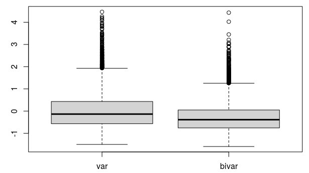
The problem, however, is that the midvariance is biased because it is based on the median and not the mean. In the example above, it is too small, whereas the empirical variance is unbiased. For small sample sizes, the bias in this example is overcompensated by the smaller variance which results in a smaller error, as you can see in the following boxplot for the 10000 simulated values for var and bivar.

boxplot(data.frame(var=x.var-sigma2, bivar=x.bivar-sigma2))

This no longer holds, however, for greater sample sizes, because the midvariance is (presumably) not even asymptotically unbiased, which means that at some size n the empirical variance starts to have a lower MSE. For n=200, I obtain:

          mean        MSE       MAE
var   1.758878 0.06049765 0.1953372
bivar 1.502718 0.10499533 0.2803434

Lax apparently sidestepped this problem by only considering symmetric distributions, which means that mean and median are the same.

Answer 2

If we assume that the underlying distribution is normal, than MAD and variance are related as $$ \hat{\sigma}=k\text{MAD}, k\approx 1.4826 $$

Mean absolute deviation (MAD) is defined as the median of the absolute deviation from the sample median. If the underlying distribution is normal, then the median is an estimator for mean and MAD, scaled as above, can serve as an estimate for the scale (i.e., \sigma$). However, unlike sample mean and sample variance, median and MAD are robust estimators of location and scale (respectively), that is they are less distorted by the outliers that might contaminate the data.

See, e.g., Robust Statistics: Theory and Methods

Answer 3

In a certain sense (unbiased minimum variance) you can't really do better than the estimator you gave above, you are efficiently using the information available in the data you are analyzing. How you can do better is e.g. if you have prior information by using a Bayesian approach or via shrinkage approaches (either sort of Bayesian shrinking towards a sensible guess, or via a hierarchical model across related quantities e.g. estimating variances for the same variable in different populations or something like that).