Get your data into a format like this:
days group  n   y
1   Control 50  3
1   Treat   50  2
2   Control 50  6
2   Treat   50  5
3   Control 50  8
3   Treat   50  23
Here days measure how long users have been in the test, n is the sample size for that group, and y is the total count of 1+ conversions. For example, the last row has 50 treated users that have been in the test for three days, and 23 have made at least one purchase. The longer you run the test, the more rows you will have.
Fit a Poisson model of y on group as a factor with a logarithmic offset equal to n*days. This will adjust for how long users have been in the test. I would use heteroskedastic variance here.
Calculate a finite difference for group from the Poisson model with the offset set to 30*N to get the effect of assigning everyone in your test to treatment for 30 days. N is the total number of users in the trial. This is not the only counterfactual for N that makes sense.
Here's an example in Stata:
. /* Parameters */
. scalar test_days         = 49

. scalar daily_inflow  = 100

. scalar frac_treat        = 2/3

. scalar p_c                       = 0.05

. scalar p_t                       = 0.10

. scalar cf_days       = 30

. scalar cf_log_offset = ln(scalar(cf_days)*scalar(daily_inflow))

. scalar true_diff         = scalar(cf_days)*scalar(daily_inflow)*(scalar(p_t) - scalar(p_c))

. /* Data */
. set obs `=scalar(test_days)'
Number of observations (_N) was 0, now 49.

. set seed 9924

. gen test_day = _n

. gen n_c          = round(scalar(daily_inflow)*(1 - scalar(frac_treat)),1)

. gen n_t          = round(scalar(daily_inflow)*scalar(frac_treat),1)

. gen y_c          = rpoisson(test_day*scalar(p_c)*n_c)

. gen y_t          = rpoisson(test_day*scalar(p_t)*n_t)

. reshape long n_ y_, i(test_day) j(group,string)
(j = c t)

Data                               Wide   ->   Long
-----------------------------------------------------------------------------
Number of observations               49   ->   98
Number of variables                   5   ->   4
j variable (2 values)                     ->   group
xij variables:
                                n_c n_t   ->   n_
                                y_c y_t   ->   y_
-----------------------------------------------------------------------------

. rename (*_) *

. strrec group ("c" = 0 "Control") ("t" = 1 "Treat"), replace
group
(49 real changes made)
(49 real changes made)

. xtset group test_day

Panel variable: group (strongly balanced)
 Time variable: test_day, 1 to 49
         Delta: 1 unit

. /* Models */
. gen double log_offset = ln(n*test_day)

. constraint define 1 _b[log_offset] = 1

.
. forvalues d = 7(7)49 {
  2.         di "Model for `d' Days"
  3.         qui poisson y i.group c.log_offset if test_day <= `d', vce(robust) constraint(1) nolog
  4.         margins, dydx(group) at(log_offset == `=ln(scalar(cf_days)*scalar(daily_inflow))') post
  5.         eststo D`d', title("`d' Days")
  6. }
Model for 7 Days

Conditional marginal effects                                Number of obs = 14
Model VCE: Robust

Expression: Predicted number of events, predict()
dy/dx wrt:  1.group
At: log_offset = 8.006368

------------------------------------------------------------------------------
             |            Delta-method
             |      dy/dx   std. err.      z    P>|z|     [95% conf. interval]
-------------+----------------------------------------------------------------
       group |
      Treat  |   168.8312   31.84171     5.30   0.000     106.4226    231.2398
------------------------------------------------------------------------------
Note: dy/dx for factor levels is the discrete change from the base level.
Model for 14 Days

Conditional marginal effects                                Number of obs = 28
Model VCE: Robust

Expression: Predicted number of events, predict()
dy/dx wrt:  1.group
At: log_offset = 8.006368

------------------------------------------------------------------------------
             |            Delta-method
             |      dy/dx   std. err.      z    P>|z|     [95% conf. interval]
-------------+----------------------------------------------------------------
       group |
      Treat  |   174.7238   17.81522     9.81   0.000     139.8066     209.641
------------------------------------------------------------------------------
Note: dy/dx for factor levels is the discrete change from the base level.
Model for 21 Days

Conditional marginal effects                                Number of obs = 42
Model VCE: Robust

Expression: Predicted number of events, predict()
dy/dx wrt:  1.group
At: log_offset = 8.006368

------------------------------------------------------------------------------
             |            Delta-method
             |      dy/dx   std. err.      z    P>|z|     [95% conf. interval]
-------------+----------------------------------------------------------------
       group |
      Treat  |   179.9386    10.7771    16.70   0.000     158.8158    201.0613
------------------------------------------------------------------------------
Note: dy/dx for factor levels is the discrete change from the base level.
Model for 28 Days

Conditional marginal effects                                Number of obs = 56
Model VCE: Robust

Expression: Predicted number of events, predict()
dy/dx wrt:  1.group
At: log_offset = 8.006368

------------------------------------------------------------------------------
             |            Delta-method
             |      dy/dx   std. err.      z    P>|z|     [95% conf. interval]
-------------+----------------------------------------------------------------
       group |
      Treat  |   154.2434   9.179377    16.80   0.000     136.2521    172.2346
------------------------------------------------------------------------------
Note: dy/dx for factor levels is the discrete change from the base level.
Model for 35 Days

Conditional marginal effects                                Number of obs = 70
Model VCE: Robust

Expression: Predicted number of events, predict()
dy/dx wrt:  1.group
At: log_offset = 8.006368

------------------------------------------------------------------------------
             |            Delta-method
             |      dy/dx   std. err.      z    P>|z|     [95% conf. interval]
-------------+----------------------------------------------------------------
       group |
      Treat  |   148.5322   7.057732    21.05   0.000     134.6993    162.3651
------------------------------------------------------------------------------
Note: dy/dx for factor levels is the discrete change from the base level.
Model for 42 Days

Conditional marginal effects                                Number of obs = 84
Model VCE: Robust

Expression: Predicted number of events, predict()
dy/dx wrt:  1.group
At: log_offset = 8.006368

------------------------------------------------------------------------------
             |            Delta-method
             |      dy/dx   std. err.      z    P>|z|     [95% conf. interval]
-------------+----------------------------------------------------------------
       group |
      Treat  |   148.9622   5.317085    28.02   0.000     138.5409    159.3835
------------------------------------------------------------------------------
Note: dy/dx for factor levels is the discrete change from the base level.
Model for 49 Days

Conditional marginal effects                                Number of obs = 98
Model VCE: Robust

Expression: Predicted number of events, predict()
dy/dx wrt:  1.group
At: log_offset = 8.006368

------------------------------------------------------------------------------
             |            Delta-method
             |      dy/dx   std. err.      z    P>|z|     [95% conf. interval]
-------------+----------------------------------------------------------------
       group |
      Treat  |   151.9719   4.731076    32.12   0.000     142.6991    161.2446
------------------------------------------------------------------------------
Note: dy/dx for factor levels is the discrete change from the base level.

. coefplot D*, pstyle(p1) xline(`=scalar(true_diff)') xlab(#15) ylab(none) title("Change in D`=scalar(cf_days)' Conversions Using D* Model") xtitle("D`=scalar(cf_days)' C
> onversions") asequation eqstrict legend(off)
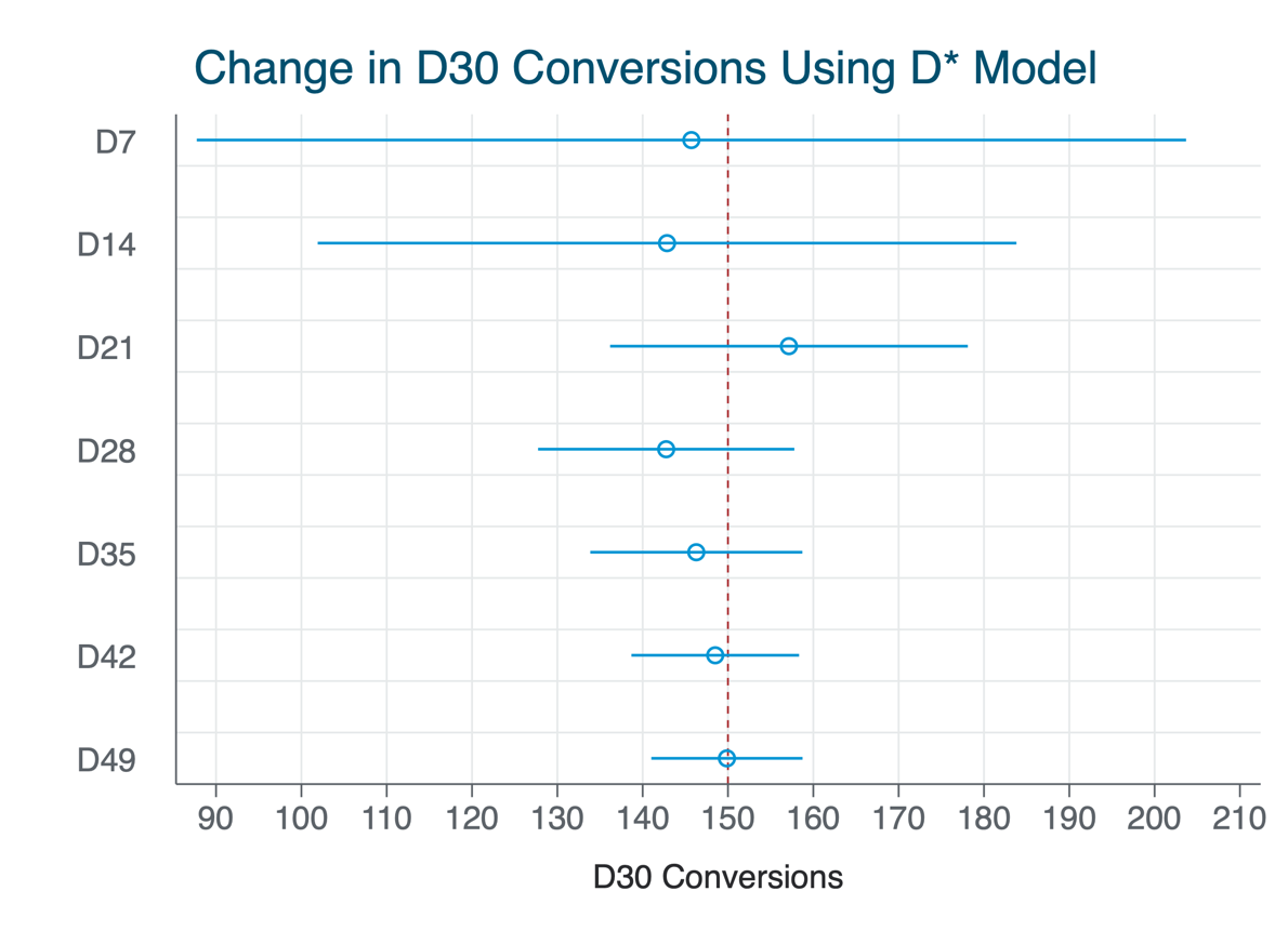
This code fits a sequence of models using 1-7 weeks of rolling test data using simulated data. Here's the graph of the total effect. :

This compares the number of conversions in 30 days if 100 users received treatment versus if they all were assigned to the control experience. The vertical line is the simulated truth. The model is able to extrapolate to 30 days fairly well using fewer than 4 weeks of data.

