5
$\begingroup$

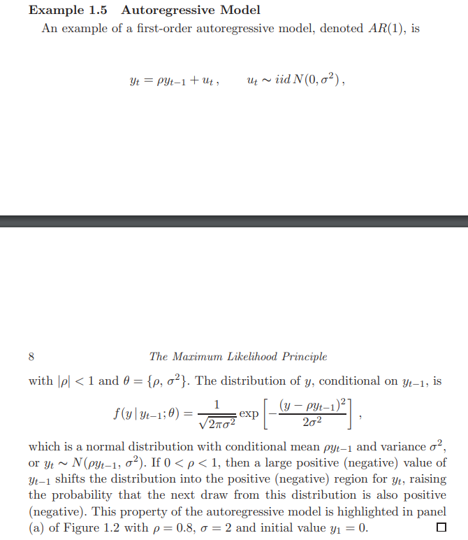
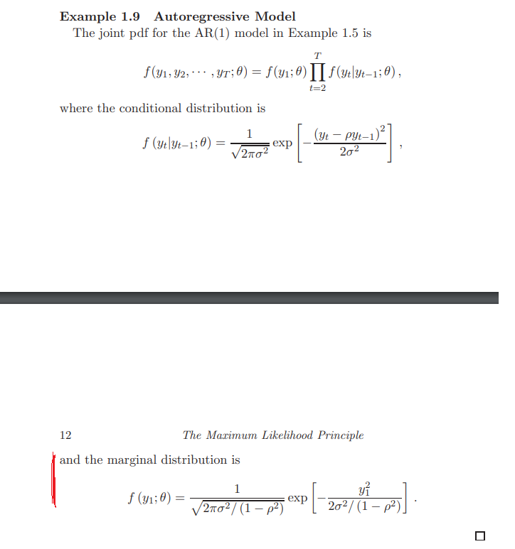
I'm reading "Econometric Modelling with Time Series" by V. L. Martin, A. S. Hurn and D. Harris ( https://www.researchgate.net/file.PostFileLoader.html?id=56bccdaa6225ff0de28b45a6&assetKey=AS:328005403594753@1455213991422 ). I don't understand example 1.9 at page 11.

Let's consider an AR(1) model : $Y_t = \rho*Y_{t-1} + \upsilon_t$ $,$ $$\upsilon_t \sim i.i.d.\text{N} \Big( 0, \sigma^{2}\Big),$$ $$|\rho|<1$$

Why is the marginal distribution of $Y_1 \sim \text{N} \Big( 0, \frac{\sigma^2}{1-\rho^2} \Big)$ ?

Thanks for your help!

Here the mentioned exampleenter image description here enter image description here

$\endgroup$
1
  • 1
    $\begingroup$ How is $Y_0$ distributed? $\endgroup$
    – mhdadk
    Commented Jan 28, 2023 at 0:32

2 Answers 2

6
$\begingroup$

This is a good technical question. Without being given the initial distribution of $Y_0$, the rigorous proof of this well-known result actually requires advanced probability theory. For the sake of rigor, we need to assume $t$ ranges over $t = 0, \pm 1, \pm 2, \ldots$.

Suppose $|\rho| < 1$, Example 3.1.2 in Time Series: Theory and Methods (2nd Edition) by Peter J. Brockwell and Richard A. Davis shows that \begin{align} X_k := \sum_{j = 0}^k\rho^jv_{1 - j} \end{align} converges to $Y_1$ almost surely. Hence to determine the (marginal) distribution of $Y_1$, it suffices to determine the limiting distribution of $X_k$ as $k \to \infty$. Clearly, being the linear combination of independent Gaussian random variables $\{v_1, v_0, \ldots, v_{1 - k}\}$, $X_k$ also follows Gaussian distribution with mean $0$ and variance $\sigma_k^2 := \sigma^2\sum_{j = 0}^k \rho^{2j} = \frac{(1 - \rho^{2(k + 1)})\sigma^2}{1 - \rho^2}$, which implies that the distribution function of $X_k$ equals to $F_{X_k}(x) = \Phi(x/\sigma_k)$, where $\Phi$ is the CDF of $N(0, 1)$. Define $\tau^2 := \frac{\sigma^2}{1 - \rho^2} = \lim\limits_{k \to \infty}\sigma_k^2$. It then follows by the continuity of $\Phi$ that $F_{X_k}(x) \to \Phi(x/\tau)$ as $k \to \infty$ for all $x \in \mathbb{R}$, which by definition means $X_k$ converges in distribution to $N(0, \tau^2)$. This proves the distribution of $Y_1$ is $N(0, \tau^2)$.

$\endgroup$
2
  • $\begingroup$ Rigorous and complete. And better framed. +1. $\endgroup$ Commented Jan 28, 2023 at 3:52
  • $\begingroup$ Thank you very much! $\endgroup$
    – andreat
    Commented Jan 28, 2023 at 11:23
2
$\begingroup$

Consider the $\sf AR(1) $ model: $$ Y_t= c+\rho Y_{t-1}+v_t.\tag 1$$ For $|\rho|< 1,$ the process is covariance stationary and the stable solution is $$Y_t = \sum_{j\in \mathbb N\cup \{0\}}[\rho^j c +\rho^jv_{t-j}].\tag 2\label 2$$ From $\eqref 2,$ it can be easily deduced \begin{align}\mathbb EY_t&=\frac{c}{1-\rho}\tag{3.1},\\\mathbb VY_t&= \frac{\sigma^2}{(1-\rho^2)}\tag{3.2}\end{align}

Since $\langle v_t\rangle$ is Gaussian, $Y_1$ is also Gaussian. Therefore, for $c=0, ~Y_1\sim\mathcal N(0,\sigma^2/(1-\rho^2).$


Reference:

$[\rm I]$ Time Series Analysis, James D. Hamilton, Princeton University Press, $1994, $ sec. $5.2, $ p. $118.$

$\endgroup$

Your Answer

By clicking “Post Your Answer”, you agree to our terms of service and acknowledge you have read our privacy policy.

Not the answer you're looking for? Browse other questions tagged or ask your own question.