One-way ANOVA F-test is significant but none of the Tukey pairwise test is significant

Question

I made up this example myself: Three geoscientists from China, USA and Europe were interested in exploring the mineralogical and textural characteristics and organic carbon composition of carbonate concretions. A concretion is a hard, compact mass of matter formed by the precipitation of mineral cement within the spaces between particles and is found in sedimentary rock or soil.

They conducted Rock pyrolysis analysis of the concretions and their host shale. Their primary goal was to compare the population mean hydrogen indices (HI measured in mg/g) for the three independent regions using an Analysis of Variance (ANOVA) procedure.

They make the usual assumptions of their samples being drawn from normal populations with equal population variances. The geoscientists reached out to a Statistics Professor to help them with the analyses using a software tool. The data is stored in an Excel file (Example1.xlsx)

H0: mu1 = mu2 = mu3

Ha: At least two means differ

The critical value (CV) from the F-table for α = 0.05 is 3.403.

# install.packages("readxl")
library(readxl)

data <- read_excel("Example1.xlsx")

data

data$Country <- factor(data$Country)

boxplot(HI ~ Country, data = data, xlab="Country", ylab = "HI")

fit <- aov(HI ~ Country, data = data)

summary(fit)

At α = 0.05 since the test statistic falls in the rejection region we reject H0 and conclude at least two populations means differ. Post-hoc tests are warranted.

So I ran the Tukey's pairwise comparison using TukeyHSD() function from the stats package and the glht() function from the multcomp R package.

# Tukey's HSD

TukeyHSD(fit)

pairwise <- TukeyHSD(fit)
  
plotdata <- as.data.frame(pairwise[[1]])
plotdata$conditions <- row.names(plotdata)

library(ggplot2)
ggplot(data=plotdata, aes(x=conditions, y=diff)) +
  geom_errorbar(aes(ymin=lwr, ymax=upr, width=.2)) +
  geom_hline(yintercept=0, color="red", linetype="dashed") +
  geom_point(size=3, color="red") +
  theme_bw() +
  labs(y="Difference in mean levels", x="",
       title="95% family-wise confidence level") +
  coord_flip()

# Multiple comparisons the multcomp package

library(multcomp)
tuk <- glht(fit, linfct = mcp(Country = "Tukey"))
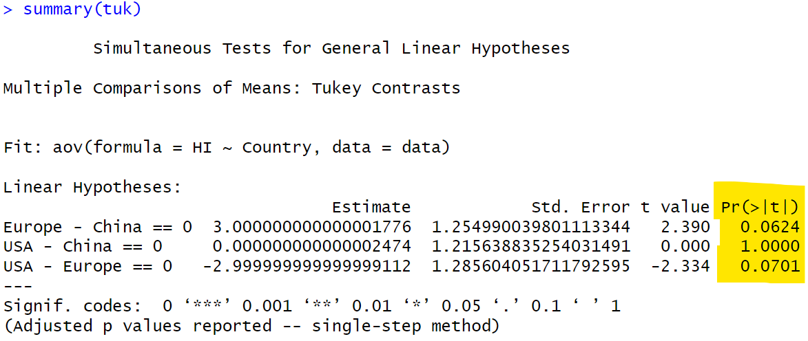
summary(tuk)

In both cases none of the pairwise test is significant. What is happening here? The fact that the main ANOVA test rejects the Ho shouldn't there be at least one significant test in the pairwise comparisons?

In other words, all group means are statistically indistinguishable from each other and can be considered to be equivalent. This result indicates that there is no evidence of significant differences in the population means of the three groups with respect to the variable being studied. Doesn't the absence of significant differences necessarily mean that the means are exactly equal in the population?

Answer 1

It is certainly plausible to have a significant omnibus test ANOVA and non-significant pairwise comparisons. This is because the ANOVA is more sensitive to overall variance across groups, as it literally accounts for the mean sum of squares for all of the grouping variables as shown by the below formula:

$$ F = \frac{\text{mean sum of squares between}}{\text{mean squares of errors}} $$

Imagine, for example, that you extract the mean sum of squares for 200 countries. This will likely result in a a lot of fluctuation, even if the actual differences between countries isn't that extreme. Pairwise tests by comparison only check comparisons between two distinct groups by using an adjusted t-test, thus only checking differences between two groups, which can sometimes account for less observed variation. As this is the case, you can have a case where the overall effect is significant because there is greater fluctuation across the spectrum of group scores but pair-by-pair they still don't vary enough to be "that big" a difference for each.

To summarize, they are two different things and can be treated as such.