14
$\begingroup$

So assuming that there is a point in testing the normality assumption for anova (see 1 and 2)

How can it be tested in R?

I would expect to do something like:

## From Venables and Ripley (2002) p.165.
utils::data(npk, package="MASS")
npk.aovE <- aov(yield ~  N*P*K + Error(block), npk)
residuals(npk.aovE)
qqnorm(residuals(npk.aov))

Which doesn't work, since "residuals" don't have a method (nor predict, for that matter) for the case of repeated measures anova.

So what should be done in this case?

Can the residuals simply be extracted from the same fit model without the Error term? I am not familiar enough with the literature to know if this is valid or not, thanks in advance for any suggestion.

$\endgroup$

5 Answers 5

6
$\begingroup$

You may not get a simple response to residuals(npk.aovE) but that does not mean there are no residuals in that object. Do str and see that within the levels there are still residuals. I would imagine you were most interested in the "Within" level

> residuals(npk.aovE$Within)
          7           8           9          10          11          12 
 4.68058815  2.84725482  1.56432584 -5.46900749 -1.16900749 -3.90234083 
         13          14          15          16          17          18 
 5.08903669  1.28903669  0.35570336 -3.27762998 -4.19422371  1.80577629 
         19          20          21          22          23          24 
-3.12755705  0.03910962  2.60396981  1.13730314  2.77063648  4.63730314 

My own training and practice has not been to use normality testing, instead to use QQ plots and parallel testing with robust methods.

$\endgroup$
4
  • $\begingroup$ Thank you Dwin. I wonder which of the different residuals should be explored (besides the Within one). Cheers, Tal $\endgroup$
    – Tal Galili
    Commented Jan 8, 2011 at 19:37
  • $\begingroup$ npk.aovE is a list of three elements. The first two are parameter estimates and normality is not assumed for them, so it wouldn't seem appropriate to test anything except $Within. names(npk.aovE) returns ` [1] "(Intercept)" "block" "Within"` $\endgroup$
    – DWin
    Commented Jan 8, 2011 at 19:57
  • $\begingroup$ @Dwin, could you check the last approach that trev posted (last answer)? It uses a sort of projection to calculate the residuals. It is the easiest approach for me in order to plot a graph with homogenity of varieances between the groups. $\endgroup$
    – toto_tico
    Commented Oct 25, 2015 at 22:54
  • $\begingroup$ @Dwin, also qqplot seems to only accept lm, and not aov. $\endgroup$
    – toto_tico
    Commented Oct 25, 2015 at 23:16
2
$\begingroup$

Another option would be to use the lme function of the nlme package (and then pass the obtained model to anova). You can use residuals on its output.

$\endgroup$
2
$\begingroup$

Venables and Ripley explain how to do residual diagnostics for a repeated-measures design later in their book (p. 284), in the section on random and mixed effects.

The residuals function (or resid) is implemented for the aov results for each stratum:

from their example: oats.aov <- aov(Y ~ N + V + Error(B/V), data=oats, qr=T)

To get the fitted values or residuals:

"Thus fitted(oats.aov[[4]]) and resid(oats.aov[[4]]) are vectors of length 54 representing the fitted values and residuals from the last stratum."

Importantly, they add:

"It is not possible to associate them uniquely with the plots of the original experiment."

For diagnostics, they use a projection:

plot(fitted(oats.aov[[4]]), studres(oats.aov[[4]]))
abline(h=0, lty=2)
oats.pr <- proj(oats.aov)
qqnorm(oats.pr[[4]][, "Residuals"], ylab = "Stratum 4 residuals")
qqline(oats.pr[[4]][, "Residuals"])

They also show that the model can be done using lme, as another user posted.

$\endgroup$
3
  • $\begingroup$ according to this, it should be [[3]] and not [[4]]. I tested it, and it just works for [[3]] $\endgroup$
    – toto_tico
    Commented Oct 25, 2015 at 22:51
  • $\begingroup$ Hey, I just stumpled across this thread. Do you think it would be okay to test these residuals with a normality test? F.e. Shapiro wilk test? @toto_tico $\endgroup$ Commented Mar 22, 2023 at 17:39
  • $\begingroup$ You can, but normality tests are usually quite sensitive, and Anova (e.g.) is somewhat robust against normality deviations (and there is no formal definition of "somewhat", usually the visual analysis would satisfy most people). The other problem is that normality tests would indicate that something is not normal, but not if something is normal (no statistical difference doesn't mean that there is no difference, just that you can't reject the null hypothesis of it being normal). $\endgroup$
    – toto_tico
    Commented Mar 23, 2023 at 11:49
2
$\begingroup$

Here are two options, with aov and with lme (I think the 2nd is preferred):

require(MASS) ## for oats data set
require(nlme) ## for lme()
require(multcomp) ## for multiple comparison stuff

Aov.mod <- aov(Y ~ N * V + Error(B/V), data = oats)
the_residuals <- aov.out.pr[[3]][, "Residuals"]

Lme.mod <- lme(Y ~ N * V, random = ~1 | B/V, data = oats)
the_residuals <- residuals(Lme.mod)

The original example came without the interaction (Lme.mod <- lme(Y ~ N * V, random = ~1 | B/V, data = oats)) but it seems to be working with it (and producing different results, so it is doing something).

And that's it...

but for completeness:

1 - The summaries of the model

summary(Aov.mod)
anova(Lme.mod)

2 - The Tukey test with repeated measures anova (3 hours looking for this!!).

summary(Lme.mod)
summary(glht(Lme.mod, linfct=mcp(V="Tukey")))

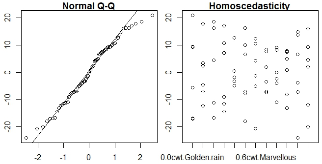
3 - The normality and homoscedasticity plots

par(mfrow=c(1,2)) #add room for the rotated labels
aov.out.pr <- proj(aov.mod)                                            
#oats$resi <- aov.out.pr[[3]][, "Residuals"]
oats$resi <- residuals(Lme.mod)
qqnorm(oats$resi, main="Normal Q-Q") # A quantile normal plot - good for checking normality
qqline(oats$resi)
boxplot(resi ~ interaction(N,V), main="Homoscedasticity", 
        xlab = "Code Categories", ylab = "Residuals", border = "white", 
        data=oats)
points(resi ~ interaction(N,V), pch = 1, 
       main="Homoscedasticity",  data=oats)

enter image description here

$\endgroup$
1
$\begingroup$

I think that the normality assumption can be assessed for each of the repeated measures, before performing the analysis. I would reshape the dataframe so that each column corresponds to a repeated measure, and then perform a shapiro.test to each one of those columns.

apply(cast(melt(npk,measure.vars="yield"), ...~N+P+K)[-c(1:2)],2,function(x) shapiro.test(x)$p.value)
$\endgroup$
3
  • $\begingroup$ Thanks gd047 - the question is what do we do when we have a more complex scenario of aov(yield ~ NPK + Error(block/(N+K)), npk) would the test you propose do the work? $\endgroup$
    – Tal Galili
    Commented Jan 8, 2011 at 20:46
  • $\begingroup$ Would you be kind enough to explain the difference between the scenarios? Unfortunately I am not familiar enough with the use of the Error term in the model (by the way, can you suggest a good book on that?). What I just proposed is the SPSS way of checking the normality assumption, as I have learned it. See this as an example goo.gl/p45Bx $\endgroup$
    – Yorgos
    Commented Jan 8, 2011 at 21:38
  • $\begingroup$ Hi gd047. Thank you for the link. The things I know about these models are all linked to from here: r-statistics.com/2010/04/… If you'll get to know of other resources - I'd love to know about them. Cheers, Tal $\endgroup$
    – Tal Galili
    Commented Jan 8, 2011 at 22:16

Your Answer

By clicking “Post Your Answer”, you agree to our terms of service and acknowledge you have read our privacy policy.

Not the answer you're looking for? Browse other questions tagged or ask your own question.