The theory behind Tukey's HSD test.

Question

I have not been able to find satisfactory explanations for the logic behind Tukey's HSD test. However, the resources I have been able to find all concern it's use. It's supposed to make multiple pairwise comparisons of means and identify those pairs which are significantly not equal.

Everything seems to hinge on the Studentized range distribution. Wikipedia says:

Suppose that we take a sample of size n from each of k populations with the same [emphasis mine] normal distribution $N(\mu,\sigma^2)$ and suppose that $y_{\min}$ is the smallest of these sample means and $y_{\max}$ is the largest of these sample means, and suppose $s^2$ is the pooled sample variance from these samples. Then the following statistic has a Studentized range distribution.

$$ q=\frac{{\overline {y}}_{\max }-{\overline {y}}_{\min }}{s/\sqrt {n}} $$

Accepting this, it would mean that assuming that all groups have identical true variance and mean, we should expect all pairwise mean differences to be smaller (in absolute value) than a certain value (which depends on our desired type 1 error significance level). However, my conclusion from this is that, in practice, if I observe that two groups have significantly different means, then the assumption that all $k$ populations have the same mean must be false. I struggle to understand how one can conclude that that specific pair of means is different?

It would make more sense to me if in the result from Wikipedia, the assumptions were relaxed so that each group could have its own mean, and the result still held.

Answer 1

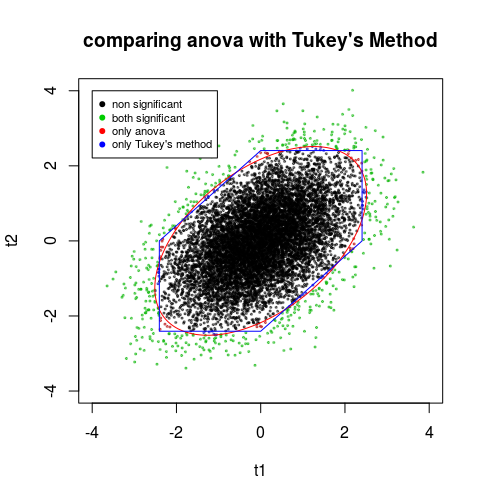
Here is a visualisation for testing the hypothesis $\mu_1 = \mu_2 = \mu_3$ which may be tested based on 3 seperate pairwise comparisons of the means by using individual t-tests based on t statistics that uses a pooled estimate for the deviation.

We simulate the distribution of the outcome of these t-tests for 3 samples of size 20 taken from a standard normal distribution. (See Comparing two, or more, independent paired t-tests) and we plot two of those t-statistics; the other is linearly dependent on the other two, $t_{1} - t_{2} + t_{3} = 0$. (Note: the signs in this linear dependency depend on how the t-statistics are computed).

What Tukey's method does, and also Anova, is defining a region such that given the hypothesis, $\mu_1=\mu_2=\mu_3$ (and the assumptions of normal distribution and equal variance), the outcome will pass some $p$ percent of the time outside the boundary. If the hypothesis is wrong then typically the outcome will be outside the boundary much more often.

Tukey's method uses the boundary based on the maximum magnitude of the t-statistics

$$q = \max(|t_1|,|t_2|,|t_3|)$$

Anova will use a boundary on the overall sizes of the t-statistics

$$F = \frac{t_1^2+t_2^2+t_3^2}{3}$$

Tukey's method will be more sensitive to situations where some $\mu_i$ are different in opposite directions (causing a large range). Anova will be more sensitive when several $\mu_i$ are different. If only a few $\mu_i$ have values at far ends, then Tukey's method will already observe a significant large distance. Anova, will be more sensitive to situations when multiple $\mu_i$ cluster at the far ends.

However, my conclusion from this is that, in practice, if I observe that two groups have significantly different means, then the assumption that all k populations have the same mean must be false.

If two means are different then the hypothesis that 'all means are the same' is obviously false, but this doesn't mean that a statement like 'some means are the same' is false. We could have the situation where two means are the same $\mu_1 = \mu_2$, and one is different from the others, $\mu_3 \neq \mu_1$ and $\mu_3 \neq \mu_2$. In such case you will get small t-statistics, except for the ones that compare with the third group. You see this in the graphic where the pointy boundary for Tukey's method extends beyond the boundary for anova when two t-statistics are extreme and the other is nearly zero (Anova is more sensitive for that case).

Answer 2

There are three possibilities

• all the means are the same
• some of the means are the same
• all the means are different

In the third case, you can't make Type I errors, because all the means are truly different, so we can ignore it.

In the first case, the studentised range distribution gives the distribution of the maximum pairwise difference, so the Type I error rate is controlled at exactly the nominal level.

In the second case, consider two means $\bar X_i$ and $\bar X_j$. If $\mu_i\neq\mu_j$ we can't make a Type I error. If $\mu_i=\mu_j$ then $\mu_i$ and $\mu_j$ are two of a set of identical means. The size of this set is less than $k$ (by assumption), so the distribution of the studentised range of this set is stochastically smaller than the studentised range of $k$ means. The Type I error is controlled conservatively.

This isn't perfect, but it's better than some older methods, which failed to control the Type I error at all in the second case.