Let $X = (X_1, ..., X_n)$ be an independent sample from $N(\mu_1, \sigma_1^2)$ and $Y=(Y_1,...,Y_m)$ an independent sample from $N(\mu_2, \sigma_2^2)$. Consider the following hypothesis test given that $\sigma_1^2 = \sigma_2^2 = \sigma^2$ is unknow. $$ H_0: \mu_1 = \mu_2 \leftrightarrow H_1: \mu_1 \neq \mu_2 $$
Notations: $\bar X$ and $\bar Y$ be the mean of sample, $\mu = \frac{n}{n+m}\bar X + \frac{m}{n+m}\bar Y$ be the pooled mean of two samples. $S_X^2 = \frac1{n-1}\sum (X_i - \bar X)^2$, $S_Y^2 = \frac1{m-1}\sum (Y_i - \bar Y)^2$, $S^2 = \frac{1}{n+m-1}\left(\sum_i (X_i -\mu)^2 + \sum_j(Y_j -\mu)^2\right)$.
Let test statistics $T_2$ be $$ T_2 = \frac{\bar X - \bar Y}{\sqrt{\frac1n + \frac1m}\sqrt{\frac{(n-1)S_X^2 + (m-1)S_Y^2}{n+m-2}}} \sim t_{n+m-2} $$ if $H_0$ is true by Cochran's theorem. The problem arises from the condition that $\sigma_1^2 = \sigma_2^2 = \sigma^2$. Let another test statistics $T_1$ be $$ T_1 = \frac{\bar X - \bar Y}{\sqrt{\frac1n + \frac1m}{S}} \sim t_{n+m-1} $$ if the $H_0$ is true. But $T_2$ is commonly used in test. My question is which is better by analyzing the power function.
To achieve that, we need to define the two different reject regions denoted $W_1$ and $W_2$ with significance level. I have done that, $$ W_1 = \{(X, Y) \big| |T_1| > t_{n+m-1}(\alpha/2) \} \\ W_2 = \{(X, Y) \big| |T_2| > t_{n+m-2}(\alpha/2) \} $$ where $t_k(\alpha/2)$ is the upper $\alpha/2$ quantile of t distribution with degree $k$.
The respect power functions are $\beta_i(\mu_1, \mu_2) = P((X, Y) \in W_i), i = 1,2$.
Assume that $(\mu_1, \mu_2)$ lies in the alternative space $\Theta_1 = \{ \mu_1\neq \mu_2 \}$, $T_2$ is a non-centralized $t$ distribution but what is the distribution of $T_1$? I got stuck here since $S$ does not obey the $\chi^2$ distribution with some degree.
Btw, the key idea of comparing two statistics is to analyze the power function. Alternative method to compare them is appreciated.
Thanks in advance.
UPDATE
This is really a question in statistics. With so many people learned about t-test during their college lectures, seldom do think deeply on conclusions they got from their textbooks.
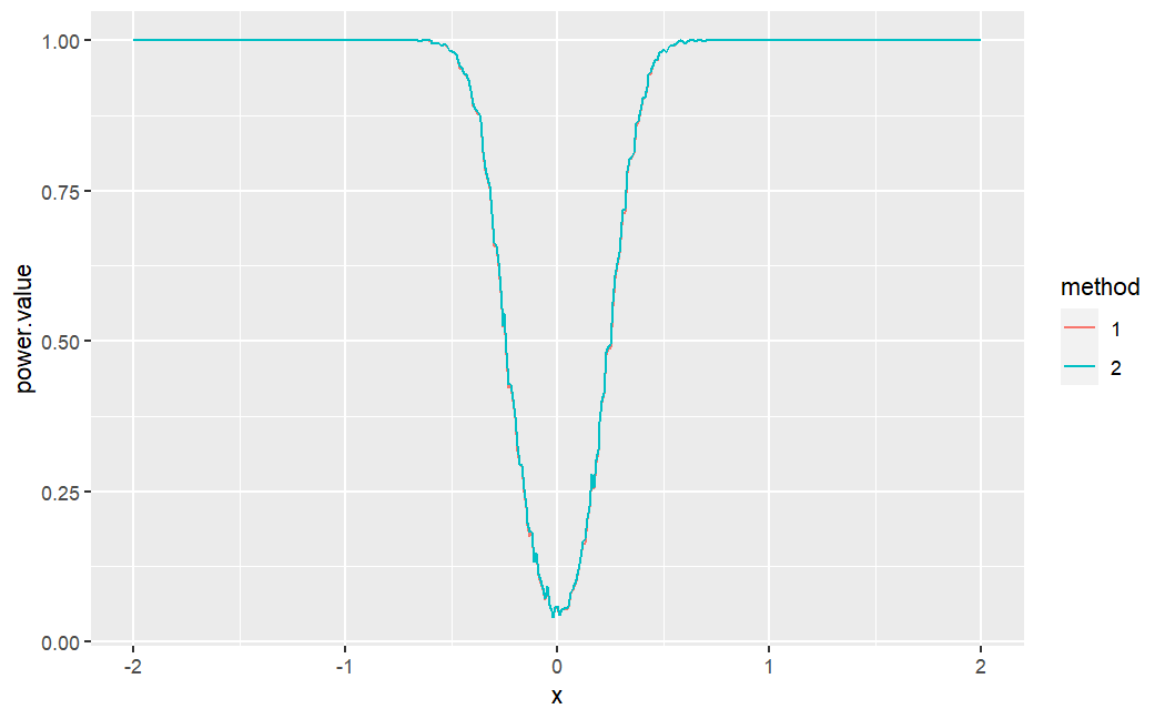
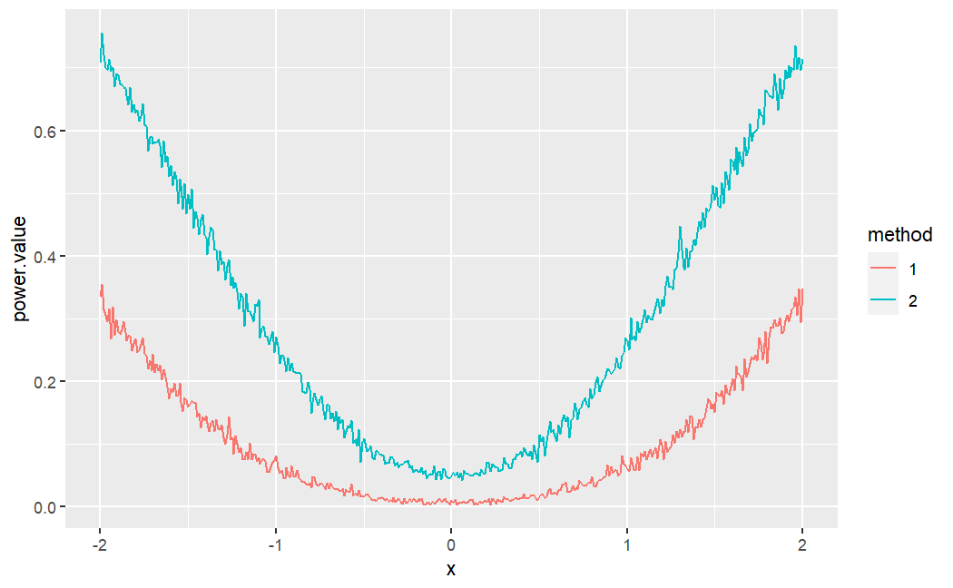
It can be seen that the real distribution of $T_2$ in $\mathcal H_1$ is noncentral student t distribution and of $T_1$, well, difficult to get. So I choose to simulate the values of power functions in R.
library(ggplot2)
delta.mu=seq(-2,2,0.01)
alpha=0.05;sigma=1
T2.fun=function(rand.x,rand.y){
  sigma_1=sqrt(((n-1)*var(rand.x)+(m-1)*var(rand.y))/(n+m-2))
  return((mean(rand.x)-mean(rand.y))/(sqrt(1/m+1/n)*sigma_1))
}

T1.fun=function(rand.x,rand.y){
  pooled.mean=mean(c(rand.x,rand.y))
  sigma_2=sqrt((sum((rand.x-pooled.mean)^2)+sum((rand.y-pooled.mean)^2))/(n+m-1))
  return((mean(rand.x)-mean(rand.y))/(sqrt(1/m+1/n)*sigma_2))
}

set.seed(1)

n=100;m=200
# reject region bound
t2=qt(1-alpha/2,n+m-2)
t1=qt(1-alpha/2,n+m-1)

pesudo.power.value1=c();pesudo.power.value2=c()
for(i in delta.mu){
  T2=c();T1=c()
  for(j in 1:1000){
    # μ1-μ2=i
    X=rnorm(n,i,sigma)
    Y=rnorm(m,0,sigma)

    T1=c(T1,T1.fun(X,Y))
    T2=c(T2,T2.fun(X,Y))
  }
  # power function value
  value1=mean(abs(T1) > t1)
  value2=mean(abs(T2) > t2)

  pesudo.power.value1=c(pesudo.power.value1,value1)
  pesudo.power.value2=c(pesudo.power.value2,value2)
}

df1=data.frame(power.value=c(pesudo.power.value1,pesudo.power.value2),
              x=delta.mu,method=gl(2,length(delta.mu)))
ggplot(df1,aes(x=x,y=power.value,color=method))+geom_smooth()

set.seed(1)
n=4;m=5
# reject region bound
t2=qt(1-alpha/2,n+m-2)
t1=qt(1-alpha/2,n+m-1)

pesudo.power.value1=c();pesudo.power.value2=c()
for(i in delta.mu){
  T1=c();T2=c()
  for(j in 1:1000){
    # μ1-μ2=i
    X=rnorm(n,i,sigma)
    Y=rnorm(m,0,sigma)

    T1=c(T1,T1.fun(X,Y))
    T2=c(T2,T2.fun(X,Y))
  }
  # power function value
  value1=mean(abs(T1) > t1)
  value2=mean(abs(T2) > t2)

  pesudo.power.value1=c(pesudo.power.value1,value1)
  pesudo.power.value2=c(pesudo.power.value2,value2)
}

df2=data.frame(power.value=c(pesudo.power.value1,pesudo.power.value2),
              x=delta.mu,method=gl(2,length(delta.mu)))
ggplot(df2,aes(x=x,y=power.value,color=method))+geom_smooth()
As you can see, in large sample size condition these two statistics are similar in test power; for a relatively small sample size, the traditional statistics we use ($T_1$) has a higher power in test. So there are reasons why we choose $T_2$: it drives $X$ and $Y$ clearly in the form of statistics which is better than take them as a whole in $T_1$.


