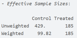
First let's talk about weighting. Weighting involves estimating a weight for each unit in the sample and then estimating the treatment effect in a way that incorproates the weights, such as weighted linear regression, weighted maximum likelihood, or a weighted difference (or ratio, etc.) in means. The weights also enter the balance statistics (e.g., standardized mean difference and KS statistics).
Separate from IPTW, it's important to understand that weighted samples have lower precision than the corresponding unweighted sample. By precision, I mean the standard error of the estimate of the desired quantity (e.g., the causal mean or difference between causal means). If we think of uncertainty arising due to the sampling of individuals, the estimate will change a lot if a unit with a large weight is swapped out for another unit in the population. Similarly, having a unit with a weight of 2 is not the same as having 2 units; choosing to use one unit's information twice doesn't give you more information about your sample; you are just changing the importance of a unit's contribution to your estimates.
The ratio of the variance (i.e., square of the standard error) of the estimate of a mean from a weighted sample to the estimate of a mean from an unweighted sample is known as the "design effect" (i.e., the effect of the "design" on the precision of the estimate) and was derived by Shook-Sa and Hudgens (2020) to be
$$
\text{deff}_w = \frac{N \sum_{i}w_i^2}{(\sum_{i} w_i)^2}
$$
where $N$ is the sample size of the group and $w_i$ is the weight for unit $i$. The effective sample size (ESS) is defined as
$$
\text{ESS} = \frac{(\sum_i w_i)^2}{\sum_i w_i^2} = \frac{N}{\text{deff}_w}
$$
and represents the size of an unweighted sample that contains the same precision as a weighted sample. When the weights are scaled to have an average of 1 (i.e., and a sum of $N$), the ESS can be equivalently written as
$$
\text{ESS} = \frac{N}{1 + \text{Var}(w^*)}
$$
where $\text{Var}(w^*)$ is the variance of the scaled weights computed using the population formula. This latter formula makes it easy to see that as the variance of the weights increases, the ESS gets smaller.
The ESS isn't the same as the sample size, but it functions like it. That is, if you have a sample of 1000 units but after weighting the sample has an ESS of 500, then you will have (approximately) the same precision as if you only had 500 units in an unweighed sample. That is the price we pay for using the weights to remove confounding. In this way, matching and weighting both function the same way, which is to trade precision for unbiasedness. The fact that weighting retains all units doesn't mean the estimates will be as precise as had you not done weighting at all; in fact, the ESS from IPTW can be smaller than the remaining sample size after matching.
The frequencies of events/conditions in the dataset is not a useful way to think about the changes caused by the weighting. The frequencies are the same as they prior to weighting; you will still have the same number of events, the same number of patients with conditions, etc., but those patients will contribute different amounts of information to the estimation of the effect and change the precision accordingly. It is useful, though, to think about weighted means and proportions of variables, since these represent balance in the weighted sample. So while the proportion of married units in one group may change from .2 to .4, that doesn't mean the actual number of married units has changed. It means the weighted sample is meant to represent a population in which 40% are married.
So, to sum up:
- The size of the weighted sample and the number of units with each condition (e.g., the number of events) is the same as the unweighted sample. Weighting does not change the sample size or number of events; it changes the relative contribution of each individual to the estimation of the treatment effect
- The effective sample size (ESS) is a measure that approximately captures the degree of precision remaining in the sample after weighting; it is not a literal sample size. It is a diagnostic statistic used for analysts to decide whether their weights have degraded their precision to an unacceptable degree. It should be reported in papers but very rarely is.
- The frequency of events is not a useful way to think about prevalence in a weighted sample. The frequency is the same in the weighted and unweighted samples, but the amount of information contained in each event changes depending on its weight. The weighted proportions/rates capture this information. Balance should be assessed on the proportion of events, not their frequency, so computing the weighted mean of a binary variable is the appropriate way to characterize prevalence after weighting, not a frequency count.

