1
$\begingroup$

My question is: what is the appropriate way to apply a kernel density estimator (KDE) to a 2D dataset that has a rotational symmetry?

Specifically, I have the points ($x_i$, $y_i$) and want the density $\rho(x,y)$. However, I know that for this system, $\mathrm{d}\rho(r, \theta)/\mathrm{d}\theta=0$ in polar coordinates. Intuitively, I should be able to use a 1D KDE to find only the radial density ($\rho(r)$) and get improved results over a 2D KDE. However, you can't just insert the radial component of the datapoints into a KDE since the 2D area scales with $r^2$ and the samples should be biased since they will be non-negative.

Some guesses for how you could proceed are to weight the datapoints with $w=1/r$. I have done this with some success for histograms before. However, I have also gotten weird artifacts when $r$ gets too close to zero. You could also replicate the datapoints with $r\to-r$ to avoid issues with the weird domain.

I couldn't find anything quickly with google'ing so it would be helpful if anyone could tell me if this has been studied before or recommend a solution / reading.

$\endgroup$
5
  • $\begingroup$ Because there is a simple relationship between the radial density and $\rho$, it really does suffice to reduce your data to a sample of $r_i$ (or some power thereof, such as $r_i^2$) and estimate its density $r$ as a 1D problem. The main complication occurs when $\rho$ is large near the origin. We have several threads about such problems. Gavin Simpson posted a powerful method at stats.stackexchange.com/a/71291/919. $\endgroup$
    – whuber
    Apr 21 at 20:34
  • $\begingroup$ @whuber, thanks! Yes, you could estimate the radial density. I am pretty worried about artifacts at r=0 though. Since $\rho(r=0)$ is nonzero in my examples, I'd have to make an estimate that goes to zero there in the right way. However, I am worried that the boundary corrections you mentioned won't guarantee the correct 2D density at the origin since it's encoding in the derivative $d\rho_r(r)/dr|_{r=0}$. Plus it would mean dividing small numbers by also increasingly small numbers as $r$ goes to zero which might have numerical issues. $\endgroup$ Apr 22 at 17:34
  • $\begingroup$ The last link I gave you will address the boundary issue at $r=0.$ Note, too, that in most cases $\rho(0)=0$ unless you have unusually high density at the origin, because the Lebesgue measure in polar coordinates is $r\mathrm dr\mathrm d\theta:$ overcoming that factor of $r$ to make $\rho(0)\ne 0$ requires your density to be singular at the origin. No standard KDE will model that very well anyway. $\endgroup$
    – whuber
    Apr 22 at 18:57
  • 1
    $\begingroup$ Yes, I did read through the link. The concern I have is that I care about an accurate prediction of the 2D distribution's density, but evaluated in polar coordinates. I can get the density of radial coordinates and I can make it go to zero using the boundary correction techniques you linked to (which, like you said, is a requirement for well-behaved distributions). However, I am worried that when I convert it back to the estimated density of the 2D distribution by dividing by $r$, that even after dealing with numerical issues of dividing by zero, the corrections won't guarantee accuracy. $\endgroup$ Apr 22 at 19:44
  • $\begingroup$ That's an excellent point -- thanks for persevering in explaining it. But why not, then, simply use KDE to estimate the density of $r^2/2$ directly rather than of $r$? And if you think the density is smooth at the origin, then applying KDE to the concatenation of $r^2$ and $-r^2$ handles the origin nicely (and automatically applies the factor of $1/2$). $\endgroup$
    – whuber
    Apr 22 at 21:58

1 Answer 1

0
$\begingroup$

I am not sure how to render this as a KDE task for practical purposes. Instead, I will propose an alternative regression type approach.

In my example, I will use a bivariate normal point cloud to get at the rotational symmetry of your problem.

$$ (x,y)\sim N(0,Diag(1)) $$

We then bin the data according to Euclidean coordinates and divide the x and y axis into bins with some equal spacing. For each bin, record the median $x,y,r,\theta$ values, and then the number of observations in each bin for a Poisson regression. In the case of the Multivariate normal I have presented above, we do not need to worry about $\theta$ because the polar representation of the the above is: $$ f(r,\theta)=\frac{1}{2\pi}r exp(-r^2/2) $$ This suggests in the log-linear regression, we need to enter $r^2$ as the relevant co-variate. Here is the implementation.

require(mvtnorm)
require(dplyr)
require(ggplot2)

set.seed(1234)
m=rep(0,2);s=diag(rep(0.1,2))
data=data.frame(rmvnorm(10000,mean = m,sigma = s))
colnames(data)<-c('x','y')
data$r<-sqrt(data$x^2+data$y^2)
data$theta<-atan(data$y/data$x)

binLim<-round(max(abs(data[,c('x','y')])))

binsize=0.1
data$x_interval<-findInterval(data$x,seq(-binLim,binLim,binsize))
data$y_interval<-findInterval(data$y,seq(-binLim,binLim,binsize))

binnedData=data%>%group_by(x_interval,y_interval)%>%summarise(
  n=n(),x=median(x),y=median(y),r=median(r),theta=median(theta)
)

binnedModel<-glm(n~I(r^2),
                 data=binnedData,
                 family=poisson)

binnedData$fitted<-binnedModel$fitted.values
plot(binnedData$fitted,binnedData$n)
binnedData$density_est=binnedData$fitted/sum(binnedData$fitted)

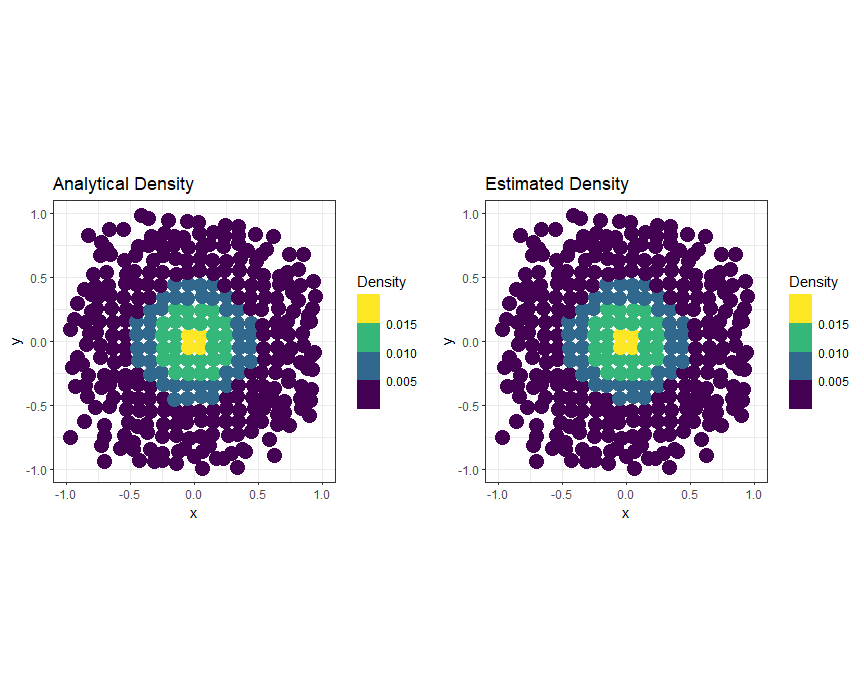
For checking against the known density function in this case: take the median values we saved and compute the integral where $b$ is the binsize used for binning the data. They seem to be roughly correct.

$$ \int_{x-b}^{x+b}\int_{y-b}^{y+b} N(0,\Sigma) $$

binnedDensities<-apply(binnedData%>%data.frame,1,function(bin){
  pmvnorm(lower = c(bin[['x']],bin[['y']])-binsize/2,
          upper = c(bin[['x']],bin[['y']])+binsize/2 ,mean = m, sigma = s)
})

ggplot(binnedData,aes(x=x,y=y))+geom_point(aes(colour=binnedDensities),size=5)+
  scale_color_viridis_b()+theme_bw()+ggtitle('Analytical Density')
ggplot(binnedData,aes(x=x,y=y,colour=density_est))+geom_point(size=5)+
  scale_color_viridis_b()+theme_bw()+ggtitle('Estimated Density')
plot(binnedData$density_est,binnedDensities)
enter image description here

$\endgroup$
4
  • $\begingroup$ (1) Aren't you making an extremely strong assumption not present in the question--namely, that the data are a sample of some bivariate Normal distribution? (2) Your examples do not exhibit the rotational symmetry assumed in the question. (3) Although it's nice to describe alternative methods of density estimation, the question really is interested specifically in (nonparametric) kernel density methods. (4) Why do you use Cartesian coordinates to create bins for an inherently polar problem? One can bin the polar coordinates just as well--and why bin $\theta$ at all? $\endgroup$
    – whuber
    Apr 21 at 20:53
  • $\begingroup$ @whuber Fair and good points. I made the initial bivariate normal assumption just to try and satisfy the rotational symmetry as I thought/recalled that the 0 mean isotropic bivariate normal has 0 dependence on $\theta$. This should render binning $\theta$ useless as I had done above and you have noted. The second example clearly violates this and should be removed, but I had included it for expounding on the idea. It probably adds more confusion than needed. I thought this might be an alternative to dealing with the non-negativity issue associated with the KDE in 1D. $\endgroup$ Apr 21 at 21:34
  • $\begingroup$ Thanks @user1848065, this is interesting, but unfortunately I deal with data that isn't well modeled by the normal distribution. It can range from uniformly distributed in 2D, to kind of gaussian looking, to even having a peak in the radial distribution somewhere that isn't $r=0$. $\endgroup$ Apr 22 at 17:38
  • $\begingroup$ @ElectronsAndStuff The method above does not technically require assumptions about the underlying distribution to work because the binned estimator is really recasting the problem as Multinomial estimation problem ... In the case of a bivariate Normal with diagonal variance 1, $r^2$ is the sufficient statistic, and I used a uniform carrying density, so everything above worked out nicely. However, this was an application of Lindsey's method for density estimation. As Gao (LinCDE) points out, you can use natural cubic splines across the domain of your values for more complex cases ... $\endgroup$ Apr 22 at 18:39

Your Answer

By clicking “Post Your Answer”, you agree to our terms of service and acknowledge that you have read and understand our privacy policy and code of conduct.

Not the answer you're looking for? Browse other questions tagged or ask your own question.