Empirical Bayes grid approximation: How to prevent the prior from overwhelming the likelihood when there are many more samples in the prior?

Question

I am trying to construct a grid approximation of the probability that an event will occur on the discrete interval 0 - 10, the spacing is 0.01. The probability that any single event on the interval is.

$$ \begin{align} p(succes|observations) &\sim Binom(n,p)\\ p &\sim Beta(a, b) \end{align} $$

Where a = number of times that the observed data was $\ge$ to a value on the interval and b = the number of times that it was not. For all values on the interval.

The observations are item counts. The observations (counts) come from many different locations. I would like to construct a grid approximation for one location given the observations from all locations.

$$ p(success\ location | all\ observations) = \frac{p(success\ location)p(all\ observations|success)}{p(all\ observations)} $$

The resulting table, where x = a value on the interval looks like this:

x	location $y \ge x$	location n	all $y \ge x$	all n
0.00	13	13	115	115
0.01	13	13	110	115
0.02	12	13	110	115
0.03	12	13	109	115

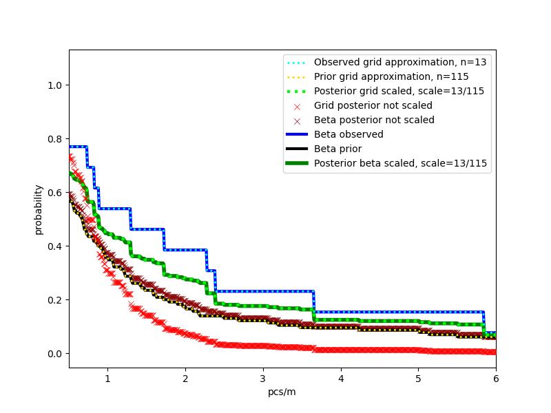
In the figure below the grid approximation was computed using Bayes theorem directly and the expected value of the beta distribution. When the prior is beta(1,1) for the beta distribution and 0.5 for Bayes theorem the expected distributions are in agreement (figure: Observed grid approximation = Beta observed and Prior grid approximation = Beta prior).

However, when the I use the posterior distribution of all observations to inform the posterior distribution of location there are two different solutions. In the first case (figure: Beta posterior not scaled), the posterior distribution of the location is pulled towards the prior (I interpret this as shrinkage). In the second case (figure: Grid posterior not scaled), the posterior distribution of location is pulled below the distribution of all observations.

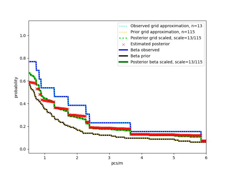
My solution: is the two distributions (figure: Posterior grid scaled, Posterior beta scaled) in green. Scaled refers to the ratio of the number of samples at the location divided by the number of all the samples: $\frac{n\ location}{n\ all}$. The beta distribution was constructed by simply multiplying the sum of the beta parameters times the scale. That is:

$$ \\ \text{from the third row of the sample table the parameters for beta are:}\\ (\alpha, \beta) = ((12, 1) + (109, 6)(\frac{13}{15})) = (24.32, 1.67)\\ \\ \text{the condtional probability is:}\\ (success, trials) = (24.32, 24.32 + 1.67) = (24.32, 26)\\ likelihood*prior = (\frac{24.32}{26})(0.5) = posterior\ distribution $$

Using this method the posterior predictive distribution is as expected. That is the posterior distribution is an average (or very close to) of the observed values at the location and the observed values from all the locations. The results are consistent for all objects (16) and locations (26).

It seems that this method is a hack even though it works very well on the defined interval using the recorded observations.

What is the correct way to achieve the desired result for the given interval?

Answer 1

Alternate Solution: There is another method that uses the parameters of the prior beta distribution and adds them to the success and trials of the likelihood. This example considers batting averages Understanding empirical Bayes estimation.

In the cited example the parameters for the beta distribution are estimated from all the data. Those estimated parameters are then added to the observed results. Which gives an approximation of the expected value of beta given the likelihood and the prior:

$$ \begin{align} S=\ \text{observed success},\ N=\ \text{trials}&, \alpha=\ \text{prior success}, \beta=\ \text{failures from prior}\\ prob(\theta)=&\frac{s + \alpha}{n + \alpha + \beta} \end{align} $$

For the use case in a grid approximation the calculation is repeated at each step in the grid. However, the magnitude of the prior is still much greater than the likelihood, the scale factor is applied to the parameters $\alpha$, $\beta$. The resulting distribution is very similar to the original solution (figure: Esitmated posterior, red x):

It is still unclear to me how to do this without creating a hierarcichal model. For this initial use case the rationale seems clear:

The influence of the prior on the likelihood should be a compromise. Scaling the parameters of the prior to the likelihood is one way to equalize the effect of one on the other.

This does have the benefit of simplicity and ease of implementation.