Finding Sample Range of Fisher's z-distribution via Approximating Hypergeometric $\,_2F_1\left(\frac{1}{2},\frac{x+1}{2};\frac{3}{2};-z^2\right)$

Question

Recently, I have encountered Hypergeometric function $\,_2 F_1\left(\frac{1}{2},\frac{x+1}{2};\frac{3}{2};-z^2\right)$ in the context of order statistics.
In particular, I am trying to evaluate an integral $n(n-1)\int _{-\infty }^{\infty } (F(d+z)-F(z))^{n-2} f(z) f(d+z) dz $,
where $F(y) = \frac{2 e^y \ _2F_1\left(\frac{1}{2},\frac{x +1}{2};\frac{3}{2};-\frac{e^{2 y}}{x}\right)}{\sqrt{x} B\left(\frac{x}{2},\frac{1}{2}\right)} = I\left({\frac{e^{2 y}}{x+e^{2 y}}};\frac{1}{2},\frac{x}{2} \right)$ to find the sample range of the Sample Range of Fisher's z-distribution with parameters $1$ and $x$.
It is known that this hypergeometric function cannot be expressed in terms of elementary functions if x is not an integer.
That said, is there a way to approximate this integral to find the distribution of the sample range?
Is there anything at all that can be said about the distribution of the sample range for Fisher's z-distribution?
What if, instead the minimum, one wants to use the median of the sample (assuming odd $n$)? Is it possible to use the connection to Beta density to find the density of$X_{(n:n)} - X_{(k:n)}$, where $k<n$, and do not evaluate integrals of the form above directly?

EDIT: The goal is to find (approximate) analytical representation of $X_{(n:n)} - X_{(k:n)}$, so one can assess its dependency on $x$ (degrees of freedom parameter)

Answer 1

Based on your goal "The goal is to find (approximate) analytical representation of X(n:n)−X(k:n), so one can assess its dependency on x (degrees of freedom parameter)" and that you are using Mathematica, an approximation to the distribution can be accomplished directly by numerical methods.

Here is the Mathematica code to find the distribution of the range for specified sample sizes and values of the degrees of freedom parameter $x$.

(* PDF of the range of n random samples from a common Fisher Z distribution with parameters 1 and x *)
pdf[d_?NumericQ, n_?IntegerQ, x_?NumericQ] := 
  NIntegrate[PDF[OrderDistribution[{FisherZDistribution[1, x], n}, {1, n}], {x1, x1 + d}],
  {x1, -\[Infinity], \[Infinity]}]

(* Plot pdf of range *)
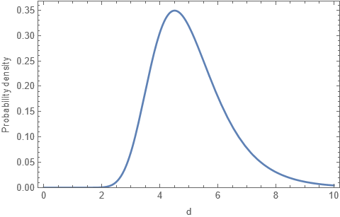
Plot[pdf[d, 30, 3.75], {d, 0, 10}, PlotRange -> {Automatic, {0, Automatic}}, Frame -> True, 
  FrameLabel -> {"d", "Probability density"}, PlotRange -> All]

(* Mean and variance of range *)
mean = NIntegrate[d pdf[d, 30, 3.75], {d, 0, \[Infinity]}]
(* 5.06407 *)
variance = NIntegrate[(d - mean)^2 pdf[d, 30, 3.75], {d, 0, \[Infinity]}]
(* 1.7515 *)

As a partial check here are simulation results with the same parameters as the above example:

(* Generate 1,000,000 samples of size 30 from a Fisher Z distribution *)
data = RandomVariate[FisherZDistribution[1, 3.75], {1000000, 30}];
(* Calculate ranges *)
range = Differences[MinMax[#]] & /@ data;
Mean[range]
(* 5.06338 *) 
Variance[range]
(* 1.75235 *)

One can investigate the relationships of various summary statistics and the degrees of freedom parameters using the above functions. (Although using simulations to do the same thing isn't much slower.)

Exact distributions

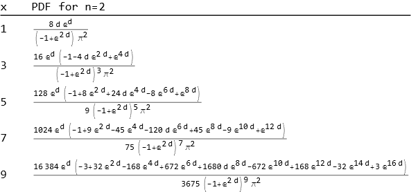
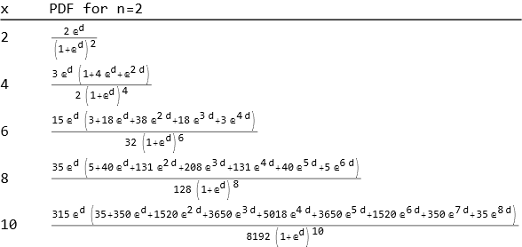
For (very) small values of $n$ (such as $n=2$), exact formulas for the pdf's, means, and variances can be obtained.

(* Fisher's z distribution functions *)
Fdz = 2 Exp[d + z] Hypergeometric2F1[1/2, (x + 1)/2, 
     3/2, -Exp[d + z]^2/x]/(Sqrt[x] Beta[x/2, 1/2]);
Fz = 2 Exp[z] Hypergeometric2F1[1/2, (x + 1)/2, 
     3/2, -Exp[z]^2/x]/(Sqrt[x] Beta[x/2, 1/2]);

(* Associated density functions *)
fz = D[Fz, z];
fdz = fz /. z -> d + z;

(* Integrand for n=2 *)
integrand = 2 fz fdz // FullSimplify;

(* Find a table of pdf's for x = 1,2,...,10 *)
pdf = FullSimplify[
   Table[{x, Integrate[integrand, {z, -\[Infinity], \[Infinity]}, Assumptions -> d > 0]},
   {x, 1, 10}], Assumptions -> z > 0 && d > 0]// TrigToExp // Together;

TableForm[pdf[[{1, 3, 5, 7, 9}]], TableHeadings -> {None, {"x", "PDF for n=2"}}]

TableForm[pdf[[{2, 4, 6, 8, 10}]], TableHeadings -> {None, {"x", "PDF for n=2"}}]

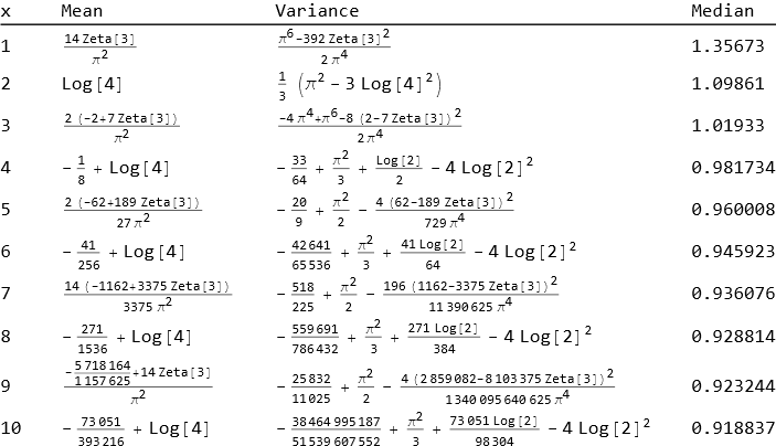
Means, variances, and medians can be obtained (although only numerically for medians):

means = Table[{x, Integrate[d pdf[[x, 2]], {d, 0, \[Infinity]}]}, {x, Length[pdf]}];
variances = Table[{x, Integrate[(d - means[[x, 2]])^2 pdf[[x, 2]], {d, 0, \[Infinity]}]},
  {x, Length[pdf]}];
medians = Table[
  {x, d /. FindRoot[CDF[ProbabilityDistribution[pdf[[x, 2]], {d, 0, \[Infinity]}], d] == 1/2,
  {d, means[[x, 2]]}]}, {x, Length[means]}] // Chop;
TableForm[Transpose[{Range[10], means[[All, 2]], variances[[All, 2]], medians[[All, 2]]}], 
  TableHeadings -> {None, {"x", "Mean", "Variance", "Median"}}]