8
$\begingroup$

I am having trouble interpreting the upper confidence interval for the odds ratio (OR) after executing Fisher's exact test in R.

I have the following contingency table which contains the response status of the subjects when given a new drug under study versus placebo:

trial_table <- matrix(c(11,5,12,19),2, 2, 
    dimnames=list(c("drug", "placebo"), c("yes","no")))

The following contingency table is then created:

        yes no
drug     11 12
placebo   5 19

I then perform base R Fisher's exact test, the alternative hypothesis being that the drug is superior to placebo.

fisher.test(trial_table, alternative = "g")

I get the following result:

    Fishers Exact Test for Count Data

data:  trial_table
p-value = 0.04949
alternative hypothesis: true odds ratio is greater than 1
95 percent confidence interval:
 1.003015      Inf
sample estimates:
odds ratio 
  3.387541

Why isn't there an upper confidence interval?

If, however, a two-sided test is performed, both lower and upper CI are reported.

    Fishers Exact Test for Count Data

data:  trial_table
p-value = 0.06871
alternative hypothesis: true odds ratio is not equal to 1
95 percent confidence interval:
  0.8298963 15.7950746
sample estimates:
odds ratio 
  3.387541 

Alternatively, I have created a bootstrap distribution for the odds ratio to get the confidence intervals (using the infer package in R), but I am not sure this is a valid approach.

The answer might be quite obvious, but not apparent to me at the moment, so I'd be grateful if someone could enlighten me.

$\endgroup$

2 Answers 2

21
$\begingroup$

There's a one-sided confidence interval because you asked for a one-sided test

$\endgroup$
7
$\begingroup$

Alternatively, I have created a bootstrap distribution for the odds ratio to get the confidence intervals (using the infer package in R), but I am not sure this is a valid approach.

Bootstrapping is often used incorrectly when used to form confidence intervals. A 95% confidence interval contains the hypothetical parameter values (odds ratios in your case) for which the p-value is above 0.05 and for which the hypothesis is not rejected.

If you use bootstrapping to compute this, then for each parameter value you would need to recompute a bootstrap sample. What is often done instead is that people compute only a single bootstrap sample and use that sample to represent the samples at other values. One must keep in mind that this is an approximation and does not work in general. See also: Why do the bootstrap calculated p-value and the confidence intervals seem to contradict each other [R code, specific example]?


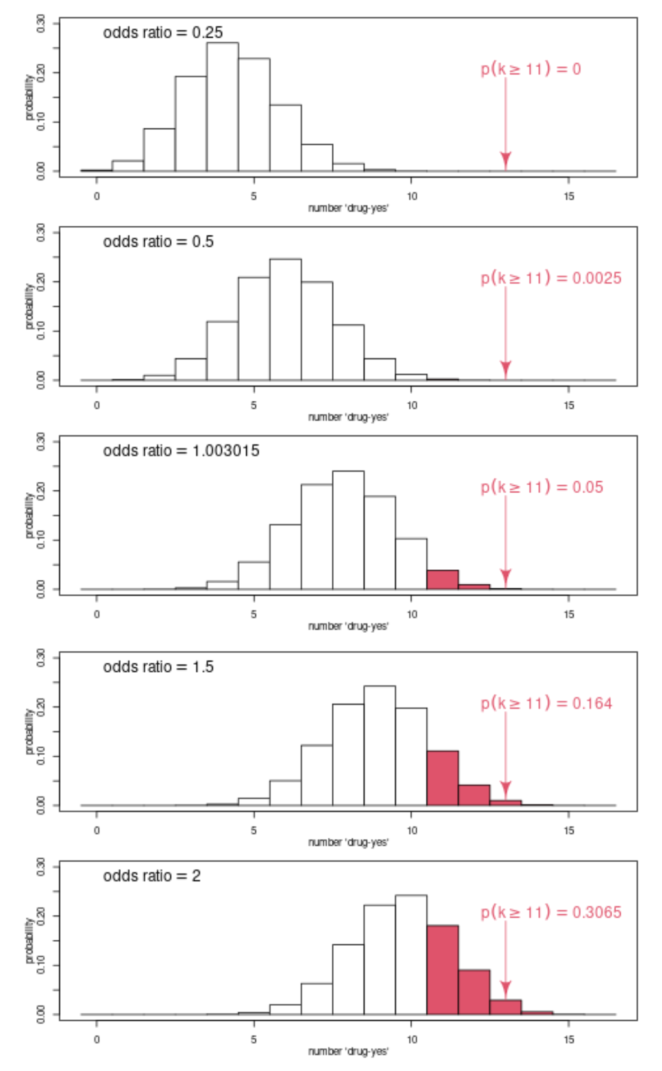
Below is an example of the distribution of observations for different hypothetical odds ratios. These distributions are computed in R with the function MCMCpack::dnoncenhypergeom

The diagrams show the probability for observing the number of 'yes' in the 'drug' group, given a certain odds ratio. For low odds ratio the probability of observing of 11 or higher is very low, and for high odds ratio this probability is higher. At odds ratio 1.003015 the probability is exactly 0.05. That's the boundary of the confidence interval. The confidence interval contains all the hypothetical odds ratio values for which the p-value is above 5%, ie for which the observation is not an unlikely value.

Because the distributions are slightly different, and not simply a shift, it can be difficult to compute only a single distribution by bootstrapping and apply it's properties to estimate the properties of all the other distributions.

example for principle behind confidence interval

Code to replicate the image:


trial_table = matrix(c(11,5,12,19),2, 2, 
    dimnames=list(c("drug","placebo"), c("yes","no")))

trial_table

fisher.test(trial_table, alternative = "g", conf.level = 0.95)

bar = function(x, h, col = 0) {
   polygon(x+c(1,1,-1,-1)*0.5,c(0,1,1,0)*h, col = col)
   return(0)
}
bar = Vectorize(bar)

for (odds in c(0.25,0.5,1.003015,1.5,2)){
  x = MCMCpack::dnoncenhypergeom(x = NA, 16, 31, 23, odds)

  plot(c(-0.5,16.5), c(-100,100), ylim = c(0,0.3), 
       xlab = "number 'drug-yes'", ylab = "probability")

  bar(0:16,x[,2], col = c(rep(0,11),rep(2,6)))

  text(0,0.28, bquote("odds ratio" == .(odds)), pos =4, font = 2, 
         cex = 1.5)
pvalue = round(sum(x[12:17,2]),4)
  text(12,0.20, bquote( p(k >= 11) == .(pvalue)  ), col = 2, pos = 4, 
       cex = 1.5)

  shape::Arrows(13,0.19, 13, x[14,2]+0.02, arr.adj = 0, col = 2)
}
$\endgroup$
3
  • $\begingroup$ I think just a layout(matrix(1:5, 5)) with five rows for each panel one was needed instead of three. $\endgroup$
    – jay.sf
    Commented Jun 26 at 10:45
  • $\begingroup$ @jay.sf this layout with 3 rows originated from my environment (I recently often use rdrr.io/snippets for images here) having standard an output of square images and puts multiple outputs on top of each other. It can be replaced with 5 rows, but it will remain dependent on the environment of the user (5 rows might cause the images to get too small and create errors/warnings as well). (often I remove any layout stuff from the posted code, also because it isn't relevant for understanding the generation of the image anyways, which is the main reason that I add such code). $\endgroup$ Commented Jun 26 at 10:52
  • $\begingroup$ I understand. I think it's cool the way it's posted now, as long as there are no errors or warnings, upvoted! $\endgroup$
    – jay.sf
    Commented Jun 26 at 11:07

Your Answer

By clicking “Post Your Answer”, you agree to our terms of service and acknowledge you have read our privacy policy.

Not the answer you're looking for? Browse other questions tagged or ask your own question.