3
$\begingroup$

I have a feeling this is a silly question. I am working on a research paper, at some point in it we perform a likelihood ratio test. The first guess would be to apply Wilks's theorem. However, if we take the hypotheses:

$$ H_0: X_i\sim Binom(n1,p1), Y_i\sim Binom(n2,p2) $$ $$ H_1: X_i\sim Binom(n1,p), Y_i\sim Binom(n2,p) $$

Essentially, we are testing wether two binomial distributions, have the same parameter $p$. Now, please do not refer me to the standard way of testing this. This is a very simplified version of the problem and in the full problem the normal approximation is inaccurate. I have found a method for the test. So while I will appreciate suggestion for actually performing the test, this is not what I am looking for here. What I am asking: Why $-2LLR$ under the null does not follow a $\chi^2_{1}$ distribution. Here is a QQplot.

I tried to find out what part of Wilks's theorem assumptions is violated here. The parameters lie in the interior of the parameter space here $(0,1)$. At this point I think that the answer must be either so obvious and I am looking too close to see the big picture, or must be some argument I don't have experience with ,either way I would like to be able to say why this is. Potentially my code is faulty. I appreciate any help/ resource I could get. Searching for papers answering this question has proven ineffective. Please be kind if this is obvious.

R code:

n1=100
n2=100

p1=0.5
p2=0.5

s=200

s1=rbinom(s,n1,p1)
s2=rbinom(s,n2,p2)


LLR= function(n1,s1,n2,s2) return(
                                  -log(choose(n1+n2,s1+s2))-((s1+s2)*log((s1+s2)/(n1+n2))+(n1+n2-s1-s2)*log(1-(s1+s2)/(n1+n2)))+
                                  (log(choose(n1,s1))+s1*log(s1/n1)+(n1-s1)*log(1-s1/n1))+
                                  (log(choose(n2,s2))+s2*log(s2/n2)+(n2-s2)*log(1-s2/n2))
                                 )

-2*LLR(n1,s1,n2,s2)


df=1

library(mgcViz)
y <- -2*LLR(n1,s1,n2,s2)
## Q-Q plot for Chi^2 data against true theoretical distribution:
qqplot(qchisq(ppoints(length(y)), df = df), y, main = expression("Q-Q plot for" ~~ {chi^2}[nu == 1]))

# Add qq line
library(ggplot2)
ggplot2::last_plot() + qqline(y, distribution = function(p) qchisq(p, df = df), prob = c(0.1, 0.6), col = 2)

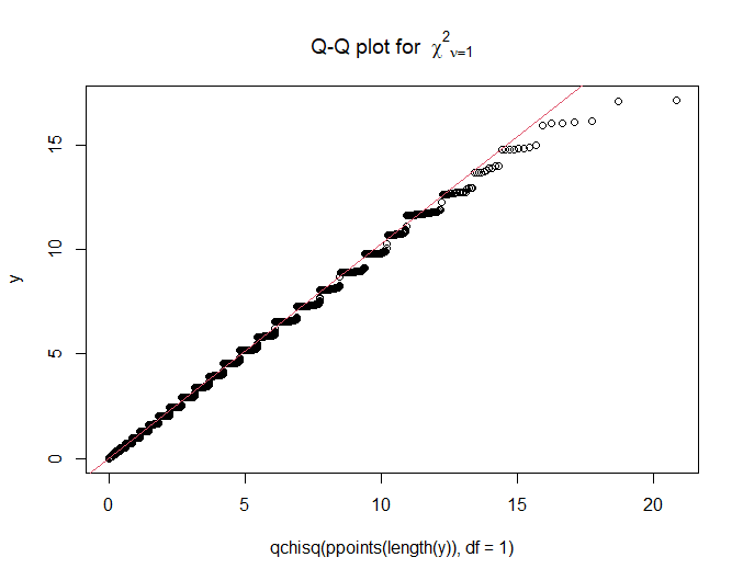
$\endgroup$
1
  • 3
    $\begingroup$ Usually the null hypothesis sets the parameters equal to each other, not the alternative hypothesis. I see in the code you set both p1=0.5 and p2=0.5 so it's not a problem in your implementation, but it might be confusing for readers to see the usual notation changed. $\endgroup$ Commented Oct 23, 2023 at 17:57

1 Answer 1

3
$\begingroup$

Your problem lies in the statement s=200; this is not a large sample size for this experiment. I've rewritten your code to make it a little clearer:

n1=100
n2=100

p <- 0.5
p1=0.5
p2=0.5

s = 100000

s1=rbinom(s,n1,p1)
s2=rbinom(s,n2,p2)

llr <- rep(0, length(s1))
  
for (i in 1:length(s1)) {
  phat0 <- (s1[i] + s2[i]) / (n1 + n2)
  llf1 <- sum(dbinom(s1[i], n1, phat0, log=TRUE)) + sum(dbinom(s2[i], n2, phat0, log=TRUE))
  phat1 <- s1[i] / n1
  phat2 <- s2[i] / n2
  llf2 <- sum(dbinom(s1[i], n1, phat1, log=TRUE)) + sum(dbinom(s2[i], n2, phat2, log=TRUE))
    
  llr[i] <- llf1 - llf2
}

y <- -2*llr

library(ggplot2)
qqplot(qchisq(ppoints(length(y)), df = 1), y, main = expression("Q-Q plot for" ~~ {chi^2}[nu == 1]))
ggplot2::last_plot() + qqline(y, distribution = function(p) qchisq(p, df = 1), prob = c(0.05, 0.95), col = 2)

With a sample size of 100,000, we get the following plot:

enter image description here

Obviously not a perfect fit, but then again, a) we are dealing with a discrete underlying distribution, and b) the result is an asymptotic one.

Is this test still useful? A quick comparison of the observed probability of rejecting the (true) null hypothesis that the two probabilities are equal:

  • $\alpha = 0.10$: observed reject rate = 0.1039
  • $\alpha = 0.05$: observed reject rate = 0.0562
  • $\alpha = 0.01$: observed reject rate = 0.0091

These are all quite close to their nominal levels, indicating that the likelihood ratio test pretty much achieves its targeted type I rejection rate. It appears to me to be a useful test, asymptotic though it is, given the sample size.

$\endgroup$
2
  • $\begingroup$ I see, however that explains why the test doesn't work, these "hitches" are substantial, is it safe to say it is a bad idea anyway? Also the tail distributions are dubious. Thank you. $\endgroup$ Commented Oct 23, 2023 at 23:55
  • $\begingroup$ I've added a paragraph to address this point. The test works fine; those hitches are really quite small, and a half dozen observations in the tail with 100,000 overall observations don't really matter. $\endgroup$
    – jbowman
    Commented Oct 24, 2023 at 0:34

Your Answer

By clicking “Post Your Answer”, you agree to our terms of service and acknowledge you have read our privacy policy.

Not the answer you're looking for? Browse other questions tagged or ask your own question.