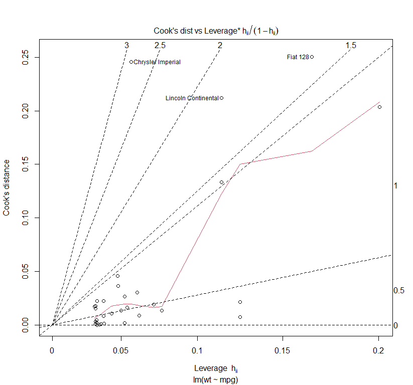
One of the R plots for a diagnostic of linear model lm() is a plot Cook's distance vs. $\dfrac{h_{ii}}{1 - h_{ii}}$. My question is: why don't we plot Cook distance against $h_{ii}$? What's the gain from $\dfrac{h_{ii}}{1 - h_{ii}}$? Obviously it is a monotonic transformation $[0,1) \mapsto [0, +\infty)$.
1 Answer
If you mean the plot, e.g.:
lm(wt ~ mpg, mtcars) |> plot(which = 6)
"I don't really see clear reason other than the fact that it exaggerates the quantity of the leverage ($h_{ii}$)" and that is what you would think on hindsight.
We know Cook's distance is a way to measure the influence of a point in the parameter estimation.
With this idea, the plot tells us whether the point has a very large influence (Cook's Distance) because of the point having a large leverage ($h_{ii}$).
And why are we looking at $\frac{h_{ii}}{1-h_{ii}}$ instead of $h_{ii}$ directly?
Well the formula of the Cook's Distance from its definition is: $$ D_i=\frac{(\hat\beta_{(i)}-\hat\beta)^\top X^\top X(\hat\beta_{(i)}-\hat\beta)}{(k+1)s^2} $$ (which is similar to euclidean distance on the estimates before and after removing a specific datapoint indexed at $i$.)
and a computational shortcut of this formula is $$D_i=\frac{r_i^2}{k+1}\left(\frac{h_{ii}}{1-h_{ii}}\right)$$
So the plot really does shows us the Cook's distance and if it is large just because of a large factor $\frac{h_{ii}}{1-h_{ii}}$ (which is again just a transformation on the leverage, $h_{ii}$)
Further reading is on chapter 9, Model Validation and Diagnostics, of Linear Models in Statistics by Rencher.

