At the outset, note that you are specifying $1+2+3+\cdots + K = O(K^2)$ parameters for this distribution, so the very best solution will require $O(K^2)$ calculations. It will also require $O(K)$ storage because there are $K+1$ possible counts.
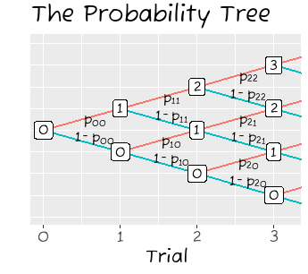
That can be accomplished by working directly through the probability tree (part of which is shown in the figure), from left to right. At stage $i$ you will have already computed the (marginal) distribution of the counts $n=0, 1, \ldots, i-1.$ Call these chances $q_{i,n}.$ The chance that the count after trial $i$ equals $n^\prime$ is the sum of the the chance there was another success after observing $n^\prime - 1$ successes or there was a failure after observing $n^\prime$ successes,
$$q_{i+1,n^\prime} = q_{i, n^\prime - 1} p_{i,n^\prime-1} + q_{i, n^\prime} (1 - p_{i,n^\prime}).$$
That is a constant amount of calculation for each of the $p_{i,n},$ the best possible. Moreover, it achieves the minimum storage requirement by needing only $K+1$ working storage.

The $q_i$ are the distributions of total successes after trial $i=0, 1, 2, \ldots.$ The values of $n^\prime$ are shown within the white boxes. The algorithm sweeps from left to right across the tree, computing the distribution at trial $i+1$ from the distribution already computed at trial $i$ based on the probabilities labeled on the connecting segments.
You could write this as a formula (it would be a product over all stages of the probability tree) but that would be less illuminating than this simple algorithm.
After performing these calculations you will have the full probability distribution and can compute any property you like. For example, the expectation of the total number of successes $N$ is (by definition)
$$E[N] = q_{K+1,0}\,0 + q_{K+1,1}\,1 + \cdots + q_{K+1,K}\,K.$$
The variance can be computed as
$$\begin{aligned}
&\operatorname{Var}(N) = \\&E[(N - E[N])^2] = q_{K+1,0}\,(0-E[N])^2 + q_{K+1,1}\,(1-E[N])^2 + \cdots + q_{K+1,K}\,(K-E[N])^2.
\end{aligned}$$
As a simple example, take $K=3$ and (using a natural vector notation) let $p_{0,*} = (1/2),$ $p_{1,*} = (1/3, 1/4),$ and $p_{2,*} = (4/5, 5/6, 6/7).$ These calculations give
$$q_{4,*} = (336, 1799, 2365, 540) / 7! \approx (0.067, 0.357, 0.469, 0.107).$$
The calculations of expectation and variance are shown at the end of the code below.
These results hold up under simulation. The appended R code performs the calculation of $q_{K+1,*}$ and runs a simulation to test it. The output for this example first compares the calculated $q$ to the simulation result (here, based on 100,000 iterations),
Method                   0     1     2     3
  q (calculated)     0.067 0.357 0.469 0.107
  q (via simulation) 0.068 0.357 0.468 0.108
The probabilities are expressed to the largest number of decimal places where close agreement can be expected. The chi-squared test of these results has a p-value of 0.48, indicating no significant difference between the calculation and the simulation.
#
# Specify the conditional distributions in the probability tree.
#
P <- list(`0` = 1/2, `1` = c(1/3, 1/4), `2` = c(4/5, 5/6, 6/7))
K <- length(P)
#
# Alternatively, specify `K` and generate random probabilities.
#
set.seed(17)
# K <- 3
# P <- setNames(lapply(seq_len(K), \(n) round(rbeta(n, 2, 2), 4)), seq_len(K) - 1)
#
# Compute the distribution of the total count.
#
q <- 1
for (i in 1:length(P)) {
  q <- c(q * (1 - P[[i]]), 0) + c(0, q * P[[i]])
}
#
#  Test with a simulation.
#
n.sim <- 1e5
N <- replicate(n.sim, {
  n <- 0
  for (p in P) n <- n + ifelse(runif(1) <= p[n+1], 1, 0)
  n
})
X <- setNames(tabulate(N + 1, nbins = K + 1), seq_len(K + 1) - 1)
#
# Compare the calculated distribution to the simulation.
#
A <- round(rbind(`q (calculated)` = q,
                 `q (via simulation)` = X / n.sim), ceiling((1 + log10(n.sim)) / 2))
names(dimnames(A)) <- c("Method", "n")
(A)
#
# Formally test the calculation.
#
chisq.test(X, p = q)
#
# Expectation and variance.
#
n <- seq_len(K+1) - 1
m <- sum(q * n)
v <- sum(q * (n - m)^2)
(c(Mean = m, Variance = v))
Edit
Here is R code to produce the illustration. It requires only that you specify a nonnegative integral value of $K$. It creates a data frame to describe the edges in the probability tree, along with consistent y coordinates for its nodes, and computes labels for the transitions. Then (using ggplot2) it describes how to render the edges and vertices of that graph. The final print command produces the figure.
#
# Describe a generic tree out to depth `K`.
#
df.tree <- function(K) {
  df.lst <- lapply(0:K, \(i) {
    data.frame(Trial = rep(i, 2 * (i + 1)),
               N = rep(0 : i, each = 2),
               N.prime = rep(0 : (i+1), each = 2)[-c(1, 2*i+4)])
  })
  X <- do.call(rbind, df.lst)
  X$Label <- apply(X, 1, \(x) paste0(ifelse(x[2] == x[3], "1 - ", ""),
                                 "p[", x[1], "*", x[2], "]"))
  X$Y <- 2 * X$N - X$Trial
  X$Y.prime <- 2 * X$N.prime - (X$Trial + 1)
  X
}
#
# Plot the (generic) tree.
# (To plot the actual tree, replace the labels by their values.)
#
X <- df.tree(K)
i.pts <- !duplicated(subset(X, select = c(Trial, Y)))

library(ggplot2)
G <- ggplot(X, aes(Trial, Y)) +
  coord_cartesian(xlim = c(-1/5, K + 1/5), ylim = c(-K-1/2, K+1/2)) +
  scale_x_continuous(breaks = seq(0, K), minor_breaks = NULL) +
  scale_y_continuous(breaks = seq(-K, K), minor_breaks = NULL) +
  ylab("") +
  geom_segment(aes(x = Trial, xend = Trial + 1,
                   y = Y, yend = Y.prime,
                   color = ifelse(N.prime > N, "Failure", "Success")),
               linewidth = 1,
               show.legend = FALSE) +
  geom_text(aes(label = Label, x = Trial + 2/3,
                y = Y + ifelse(N == N.prime, -2/5, 2/5)),
            data = subset(X, Trial < K), parse = TRUE,
            size = 20 / (K+1)) +
  geom_label(mapping = aes(label = N), data = X[i.pts, ],
             size = 20 / (K+1)) +
  theme(axis.text.y = element_blank(),
        axis.ticks.y = element_blank(),
        text = element_text(size = 14)) +
  ggtitle("The Probability Tree")

print(G)

