I think you can understand why LASSO selects at most $n$-features intuitively if you think about the contours of $rss = |X\beta - y|_2^2$ and $l_1 = |\beta|_1$ on the parameter space $\mathbb R^p$. You can think about finding the minimal $rss + l_1$ solution as looking at the 2 contours of larger and larger values for $rss$ and $l_1$ until they intersect for the first time. Their growth with respect to each other needs a specific ratio, but that's irrelevant for the intuition, in fact in your head you might want to keep the $l_1$-contour constant.
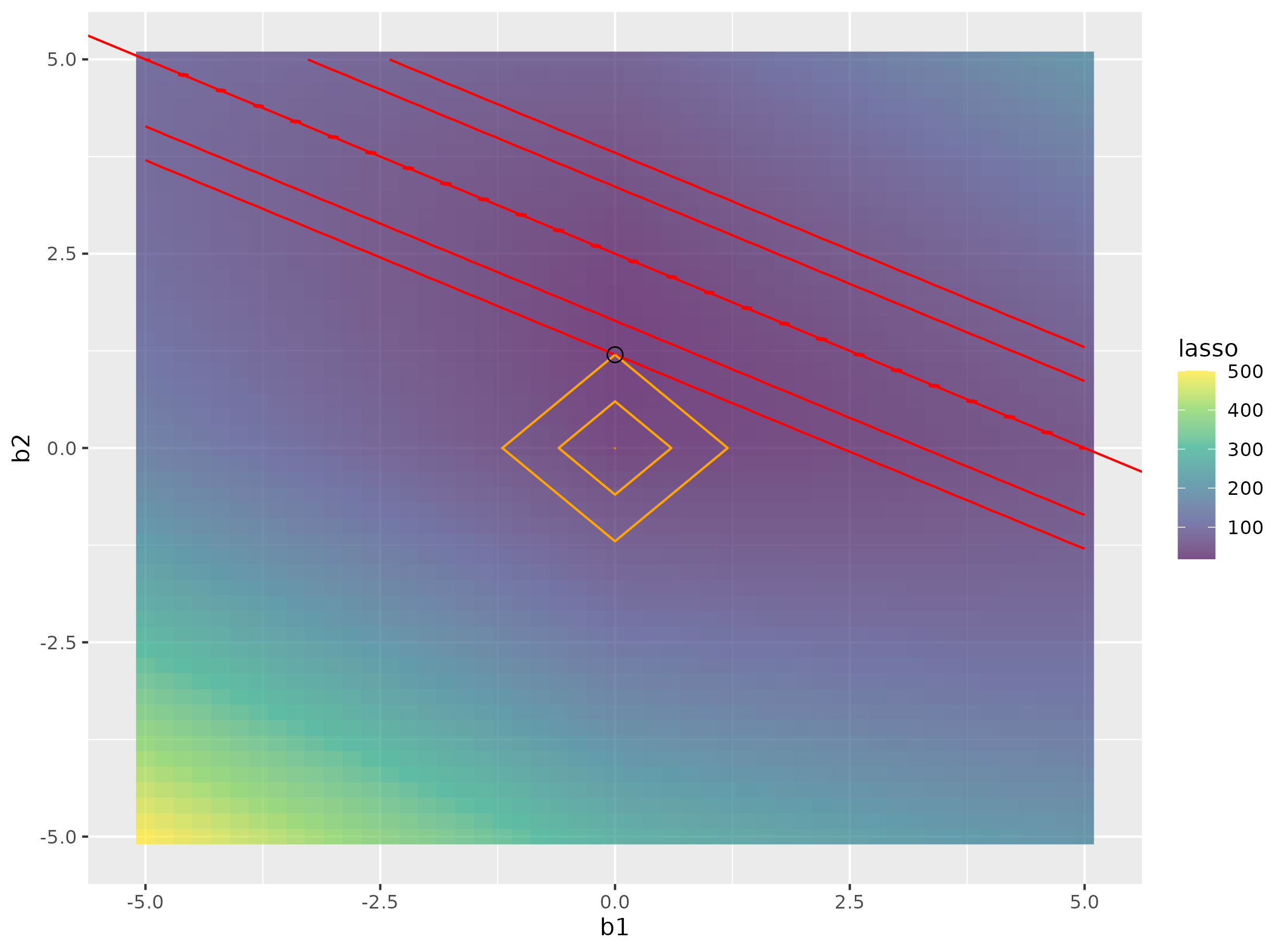
The $l_1$-contour will be a generalized octahedron (https://en.wikipedia.org/wiki/Octahedron) with the corners on the axis. For your example with $p = 2$ that's just a square with sides 45 degrees rotated against the axis. For $rss$ let's first think about $rss = 0$, so the solution space to $X\beta = y$. That's a $p-n$-dimensional affine subspace. In your example that's the line $\beta_2 = -0.5\beta_1 + 2.5$. $rss$ is just distance squared so constant $rrs \implies$ constant distance. Therefor the contours will be parallel(or a elliptic, symmetric arrangement of parallel spaces) to the original subspace.
Let's check it out in your example (R-code, at the bottom, I improved some stuff and choose $\lambda = 10$ for visibility) :
:
The solution is at $\beta_1 = 0, \beta_2 = 1.2$. In red you can see the contours of $rss$ and in orange the contours of $l_1$. The question comes down to how can the red lines be tangent to an orange square?
By going through one of the corners, which is on an axis, so the other parameter will be $0$.
By being parallel to one of the sides and touching the whole side, in which case you have non unique solutions (https://www.stat.cmu.edu/~ryantibs/papers/lassounique.pdf) This is partially discussed in some of the threads you linked. If you change $x_2 = 1$ in your example, then you will have an obvious case.
Generalizing: the $l_1$-contour is made up of $d$-dimensional edges ($d = 0$ is a corner, $d = 1$ is an edge, $d = 2$ is a 2d-surface like the face for $p = 3$, ...) and hitting that $d$-dimensional edge correspond to selecting $d+1$ features. The $rss$-contour covers $p-n$-dimension and the $n$-dimensional edge, that would select $n+1$ features, covers the remaining dimensions, so there is no space to not be parallel.
In $p = 3$ you can check this out with an 8-sided-die for the $l_1$-contour and for $n = 1$ a large piece of paper or for $n = 2$ a pencil, to stand on for the plane/lines that make up the $rss$-contours. A 6-sided-die is also fine for getting the idea.
# Implemented the fix from Eoins answer
# Comment on your Code: you are loading a library, use that for
# readability instead of andless ::
library(tidyverse)
data <- data.frame(x1 = c(1),
                   x2 = c(2),
                   y = c(5))
range <- 5
b1 <- seq(-range, range, length.out = 51)
b2 <- seq(-range, range, length.out = 51)
model <- expand.grid(b1 = b1, b2 = b2)

compute_loss <- function(model, data, lambda) {
  y_hat <- model["b1"] * data$x1 + model["b2"] * data$x2
  rss <- mean((data$y - y_hat)^2)
  l1 <- lambda * sum(abs(model))

  data.frame(rss = rss,
             l1 = l1,
             lasso = rss + l1,
             b1 = model["b1"],
             b2 = model["b2"],
             y_hat = y_hat)
}
lambda <- 10 # l1 closer to rss values
costs <- apply(model, 1, compute_loss, data, lambda) %>%
  bind_rows()
costs %>%filter(lasso == min(lasso))
# rss  l1 lasso  b1 b2   y_hat
# 6.76 12 18.76  0 1.2   2.4
# making about with the breaks argument, to show
ggplot(costs, aes(x = b1, y = b2, fill = lasso))+
  geom_raster() +
  geom_contour(aes(z = rss), breaks = c(0.01, sqrt(6.76/2), 6.76),
                     color = "red") +
  geom_abline(intercept = 2.5, slope = -0.5, color = "red", ) +
  geom_contour(aes(z = l1), breaks = c(0.01, 6, 12),
                   color = "orange") +
  geom_point(data = costs %>%filter(lasso == min(lasso)), size = 3,
              shape = 1) +
  scale_fill_viridis_c(alpha = 0.7)


