Are p-values computed from the a priori or a posteriori sampling distribution?

Question

Wikipedia defines a p-value as follows:

the p-value is the probability of obtaining test results at least as extreme as the result actually observed, under the assumption that the null hypothesis is correct.

And to compute a p-value, we need a sampling distribution.

My question is: when we talk about the null hypothesis here, are we referring to the sampling distribution constructed:

1. Before any data is collected (a priori), or
2. After data has been collected (a posteriori)?

Bonus points for providing any reference which speaks to this explicitly.

I think the correct answer is the a priori version, otherwise our type 1 and 2 error rates may deviate from the rates specified during the power analysis. However, I believe most A/B test software calculates the p-value from the sampling distribution generated directly from the sample data collected - so I'm confused.

Quick example

Suppose that I am planning to test a new website landing page, with the aim of improving conversion rates. Applying the Null Hypothesis Significance Testing framework (NHST), I lay out my hypotheses a priori:

• Null hypothesis (H₀): treatment and control samples are drawn from populations with identical proportions: 6% conversion rates
• Alternate hypothesis (H_A): treatment and control samples are drawn from populations with different proportions: 7% and 5% conversion rates, respectively

To achieve a significance level of 0.05 and a power of 0.8, I calculate a minimum required sample size of 2213:

# R code
prop_baseline <- 0.05          
prop_treatment <- 0.07
alpha <- 0.05
beta <- 0.2 

n <- ceiling(
        power.prop.test(
            p1 = prop_baseline, 
            p2 = prop_treatment, 
            sig.level = alpha, 
            power = 1-beta, 
            alternative = c("two.sided")
        )$n
      )
n

# [1]  2213

I also determine the a priori critical value (= 1.4%):

prop_pooled <- (prop_baseline+prop_treatment)/2
se_h0 <- sqrt(prop_pooled * (1-prop_pooled) * (1/n + 1/n))
se_ha <- sqrt((prop_baseline*(1-prop_baseline))/n + 
    (prop_treatment*(1-prop_treatment))/n)
critical_value <- qnorm(alpha / 2, mean = 0, sd = se_h0, 
    lower.tail = FALSE)
critical_value

# [1]  0.0139930354339993

We can visualize the sampling distributions for both hypotheses like so:

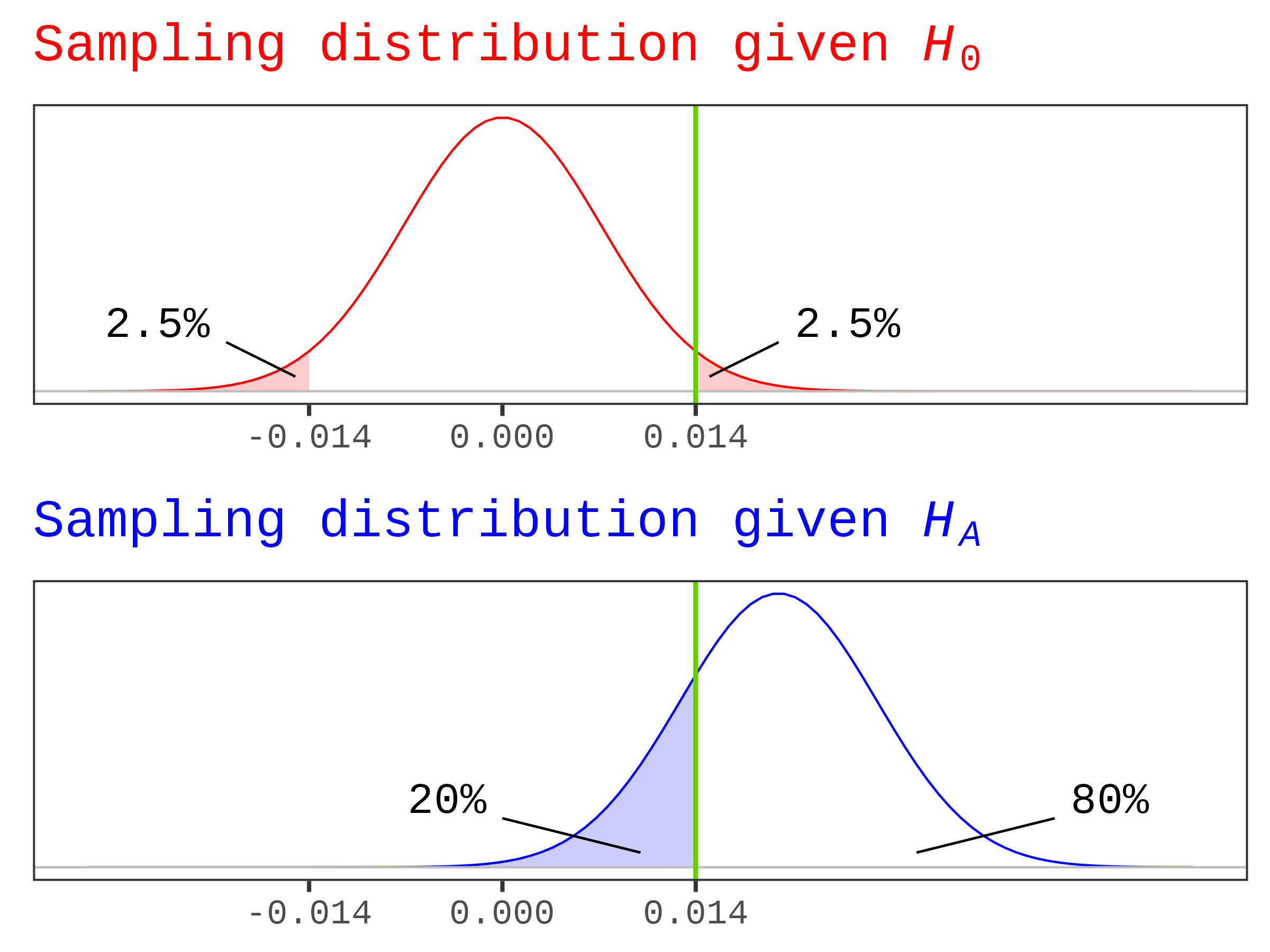
At the conclusion of the test, the results are:

The a priori decision framework:

The effect size (= 0.0154) is greater than the critical value (= 0.0140).

And so, the p-value < 0.05:

2*(1 - pnorm(0.01536376, mean = 0, sd = se_h0))

# [1]  0.0314007090609361

So, we reject the null hypothesis in favor of the alternate hypothesis.

The a posteriori decision framework:

The p-value > 0.05:

prop.test(x=c(141, 175), n=c(n,n))$p.value

# [1]  0.0540496200600176

So, we DO NOT reject the null hypothesis.

What's the correct approach?

Answer 1

The null hypothesis is fixed before looking at the sample (or even planning the sample size). The p-value is obviously computed from the data, but it is based on the test statistic, which normally compares the data with what is expected under the null hypothesis. The null hypothesis is rejected if the "distance" is too big.

Note however that in your example prop.test will test the null hypothesis that the two probabilities are the same and not necessarily 0.06. This is the reason that it doesn't rely on the critical value that you have computed for probability 0.06. So the difference between your two setups is not that one is "a priori" and the other one is "a posteriori" (these terms are not used as a standard in frequentist analyses such as hypthesis tests), but rather that your first test tests the null hypothesis that the probabilities are both equal to 0.06 (so that you can fix the standard error), whereas the second one tests the null hypothesis that both probabilities are equal and can be anything (so that the standard error needs to be estimated from the data; this is apparently what you call "a posteriori").

Both of your test results can make sense; as both relative frequencies (141/2213 and 175/2213) are larger than 0.06, it makes sense to reject the H0 that they are both 0.06, but they may still both be 0.07, say.

In order to fix the sample size in advance, you can choose some specific parameter values in order to do the calculations (you may want to reach a specific power for specific relevant choices of parameters), but given the sample sizes and the data, most tests will test more general null and alternative hypotheses against each other.

Answer 2

My question is: when we talk about the null hypothesis here, are we referring to the sampling distribution constructed:

Before any data is collected (a priori), or

After data has been collected (a posteriori)?

In a one-sample t-test, for example, it is a combination.

A priori, you decide your null hypothesis, say $\mu=0$ (in general, $\mu = \mu_0$ for some constant $\mu_0$).

A posteriori, you calculate the sample variance, the sample mean, and the sample size.

All four components go into calculating the sampling distribution, test statistic, and p-value.

$$ \dfrac{\bar X - \mu_0}{s/\sqrt{n}} \sim t_{n - 1} $$

These terms a priori and a posteriori allude to and sound like, but are not the same as, the ideas of prior and posterior distributions in Bayesian statistics.

Answer 3

The p-value is computed with the sampling distribution

Given a parameter $\theta \in \Theta$, an observed data vector $\mathbf{x}$ and a test statistic $T$ that is increasing with respect to evidence for the alternative hypothesis (i.e., a higher value is more conducive to the alternative), the p-value for the null hypothesis $H_0: \theta \in \Theta_0$ is defined as:

$$\begin{align} p(\mathbf{x}) &\equiv \sup_{\theta \in \Theta_0} \mathbb{P}(T(\mathbf{X}) \geqslant T(\mathbf{x}) | \theta) \\[12pt] &= \sup_{\theta \in \Theta_0} \ \int \limits_{\mathbf{r} : T(\mathbf{x}) \geqslant T(\mathbf{r})}^\infty f_\mathbf{X}(\mathbf{r}|\theta) \ d \mathbf{r}, \\[6pt] \end{align}$$

As you might be able to see, the p-value is a function of the sampling distribution $f_\mathbf{X}(\ \cdot \ |\theta)$. The sampling distribution is the distribution of the data vector conditional on the parameter, so it is neither the prior distribution (unconditional distribution of the parameter) nor the posterior distribution (conditional distribution of the parameter given the data) used in Bayesian statistics.

Answer 4

• The $p$-value is a posteriori because it depends on the observed data (or more precisely the observed test-statistic, $T^\star$), being $$ p = \text{Pr}(T \ge T^\star | H_0) $$

• The type-1 and type-2 error rates are a priori as the type-1 error rate is chosen by the research before collecting data and the type-2 error rate depends only on the experimental design (and the chosen type-1 error rate) and not on the observed data.

• The outcome of a null hypothesis significance test is a posteriori as the decision on whether or not to reject (at a priori chosen threshold) depends on the observed data.

Answer 5

I have caused confusion by using the terms "a priori" and "a posteriori". To acknowledge this I will use the phrases "before data collection" and "after data collection" here, instead.

In my question, I identified two separate methods for calculating a p-value (differing by standard error) and I asked which was the correct method to use. For the same set of data, each method produced a different answer and this was of concern to me.

I now believe that the two frameworks provide near identical results (validated via simulation) - it's just that in the example I provided, I had mistakenly included Yates' continuity correction in prop.test(). Once I remove this, the results are very similar:

P-value determined via the null hypothesis sampling distribution (constructed BEFORE data is collected)

prop_baseline <- 0.05          
prop_treatment <- 0.07
n <- 2213
observed_delta <- 0.01536376

print('Standard error of null hypothesis sampling distribution')
se_ha <- sqrt((prop_baseline*(1-prop_baseline))/n + (prop_treatment*(1-prop_treatment))/n)
se_ha

print('P-value')
2 * (1 - pnorm(observed_delta, mean = 0, sd = se_ha))

[1] "Standard error of null hypothesis sampling distribution"
0.00713310288729407
[1] "P-value"
0.0312505476484228

P-value determined via the null hypothesis sampling distribution (constructed AFTER data is collected)

conversions_baseline <- 141
conversions_treatment <- 175
n <- 2213
prop_pooled  <- (conversions_baseline/n + conversions_treatment/n)/2
observed_delta <- 0.01536376


print('Standard error of null hypothesis sampling distribution')
se_ha <- sqrt(prop_pooled * (1-prop_pooled) * (1/n + 1/n))
se_ha
print('P-value manual computation')
2 * (1 - pnorm(observed_delta <- 0.01536376
, mean = 0, sd = se_ha))
print('P-value prop.test computation')
prop.test(x=c(conversions_baseline, conversions_treatment), n=c(n,n), correct = FALSE)$p.value

[1] "Standard error of null hypothesis sampling distribution"
0.00774064826424033
[1] "P-value manual computation"
0.0471649830099237
[1] "P-value prop.test computation"
0.0471649887275255

Now (in contrast to the original example), both methods yield a p-value < 0.05, so we reach the same decision (to reject the null hypothesis) for this particular observation.

Globally, both methods yield very similar power estimates

set.seed(123)

#####################
# Initialize inputs
#####################
prop_baseline <- 0.05          
prop_treatment <- 0.07
alpha <- 0.05
beta <- 0.2 

n <- ceiling(
        power.prop.test(
            p1 = prop_baseline, 
            p2 = prop_treatment, 
            sig.level = alpha, 
            power = 1-beta, 
            alternative = c("two.sided")
        )$n
      )


#####################
# Generate sampling distribution under HA
#####################
num_experiments <- 10000

prop_pooled <- (prop_baseline+prop_treatment)/2
se_h0 <- sqrt(prop_pooled * (1-prop_pooled) * (1/n + 1/n))
se_ha <- sqrt((prop_baseline*(1-prop_baseline))/n + (prop_treatment*(1-prop_treatment))/n)
critical_value <- qnorm(alpha / 2, mean = 0, sd = se_h0, lower.tail = FALSE)

conversions_baseline <- replicate(num_experiments, rbinom(1, size = n, prob = prop_baseline))
conversions_treatment <- replicate(num_experiments, rbinom(1, size = n, prob = prop_treatment))
prop_delta <- conversions_treatment/n - conversions_baseline/n

#####################
# Generate p-values
#####################
p_values <- vector("numeric", length = num_experiments)
for(i in 1:num_experiments){
  p_values[i] <- prop.test(x=c(conversions_baseline[i], conversions_treatment[i]), n=c(n,n), correct = FALSE)$p.value
}

#####################
# Determine power
#####################
print('power_via_sampling_dist_before_data_collection')
power_via_sampling_dist_before_data_collection <- sum(prop_delta>critical_value)/num_experiments
power_via_sampling_dist_before_data_collection
print('power_via_sampling_dist_after_data_collection')
power_via_sampling_dist_after_data_collection <- sum(p_values<0.05)/num_experiments
power_via_sampling_dist_after_data_collection

[1] "power_via_sampling_dist_before_data_collection"
0.8109
[1] "power_via_sampling_dist_after_data_collection"
0.8068

Finally, any discrepancy almost completely disappears when we move away from "chunky binomial probabilities to smooth Gaussian distribution" as per Harvey Motulsky's comment.