Poisson regression for rare events?

Question

Poisson regression is commonly used to analyse count data. However, when we deal with rare events it does not seem to be appropriate any more. At least, graphical criteria to assess the model fit like Pearson residuals or deviance residuals are inappropriate.

How do we have to deal with that?

For example, consider the following toy example. Coefficient estimates are actually close to the ‚true‘ values which we never know, of course. So, how can we evaluate and measure the model fitness?

Edit to clarify the question: I think the significance tests for the parameter in the summary output use the the Pearson and deviance residuals, at least implicitly. So if these residuals are not appropriate in this case, how reliable are the significance tests?

# Toy-Example (Poisson Regression, Rare Event)
set.seed(11)

N <- 100000

# Two categorical variables
I1 <- sample(c(0,1), size = N, replace = TRUE)
I2 <- sample(c(0,1), size = N, replace = TRUE)


lambda <- 0.05*0.9^I1*1.2^I2

Y <- rep(0,N)

for (i in 1:N){
  
  Y[i] <- rpois(1,lambda=lambda[i])
  
}


model <- glm(Y ~ I1 + I2, family = poisson())
summary(model)

# Coefficients are close to the true values
exp(model$coefficients)

# However residuals look awful
res0 <- Y - model$fitted.values
res1 <- residuals(model, "pearson")
res2 <- residuals(model, "deviance")

par(mfrow=c(2,3))
plot(model$fitted.values,res0, main = "Raw Residuals")
plot(model$fitted.values,res1, main = "Pearson Residuals")
plot(model$fitted.values,res2, main = "Deviance Residuals")
#
boxplot(res0, main = "Raw Residuals")
boxplot(res1, main = "Pearson Residuals")
boxplot(res2, main = "Deviance Residuals")

Answer 1

Welcome to CV. Poisson regression is fine for rare events. In fact, it got started with modeling the number of soldiers kicked to death by the horses --- not common, even in the days of large cavalry forces! The problem is that the plots you made aren't great for the purpose you are using them for when you are running Poisson regression.

The patterns of residuals in the plots is due to the discrete nature of your dependent variable. This has been discussed on CV before e.g. here. A better alternative is discussed here .

Answer 2

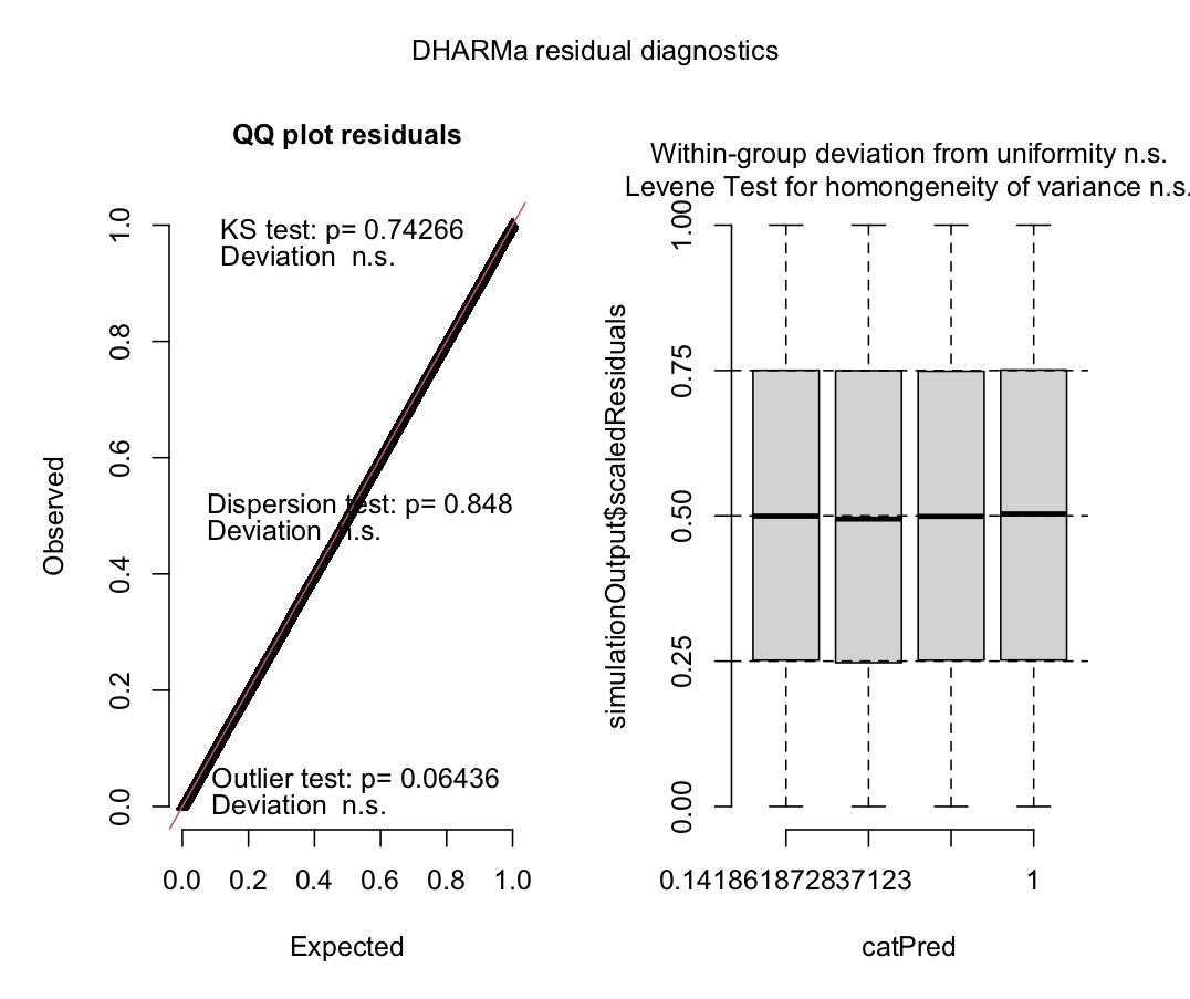
Peter Flom is correct (+1). For completeness, here's the recommended graphical evaluation of the model in the OP, following the method in this answer based on the DHARMa package. (I have version 0.4.3 installed on this computer; 0.4.6. is the current version.)

library(DHARMa)
res <- simulateResiduals(model)
plot(res)

Those residuals are certainly well behaved.

Answer 3

I agree with the answers above, but I think that there is (somehow) one point missing.

The method of Dunn and Smyth (1996) may serve as a graphical criteria, which was the main focus of the question. However, I have not found a result in their paper that makes me feel comfortable judging the sensitivity of such a graphical criterion.

In the following example (with a slightly disturbed data) the likelihood-based significance tests indicates that there is something wrong. The randomized quantile residuals seem not to be sensible to such a misspecification:

# Toy-Example (Poisson Regression, Rare Event)
set.seed(19)

N <- 10000

# Two categorical variables
I1 <- sample(c(0,1), size = N, replace = TRUE)
I2 <- sample(c(0,1), size = N, replace = TRUE)


lambda <- 0.05*0.9^I1*1.2^I2

Y <- rep(0,N)

# Error
Error <- rbinom(length(Y),1,prob=1/10)


for (i in 1:N){
  
  # Disturbance 
  Y[i] <- rpois(1,lambda=lambda[i]) + Error[i]
  
}


model <- glm(Y ~ I1 + I2, family = poisson())
summary(model)

# Mehod of Dunn and Smyth (1996)
library(DHARMa)

res <- simulateResiduals(model)
plot(res)