13
$\begingroup$

I'm coming from this question in case anybody wants to follow the trail.

Basically I have a data set $\Omega$ composed of $N$ objects where each object has a given number of measured values attached to it (two in this case):

$$\Omega = o_1[x_1, y_1], o_2[x_2, y_2], ..., o_N[x_N, y_N]$$

I need a way to determine the probability of a new object $p[x_p, y_p]$ of belonging to $\Omega$ so I was advised in that question to obtain a probability density $\hat{f}$ through a kernel density estimator, which I believe I already have.

Since my goal is to obtain the probability of this new object ($p[x_p, y_p]$) of belonging to this 2D data set $\Omega$, I was told to integrate the pdf $\hat{f}$ over "values of the support for which the density is less than the one you observed". The "observed" density is $\hat{f}$ evaluated in the new object $p$, ie: $\hat{f}(x_p, y_p)$. So I need to solve the equation:

$$\iint_{x, y:\hat{f}(x, y) < \hat{f}(x_p, y_p)} \hat{f}(x,y)\,dx\,dy$$

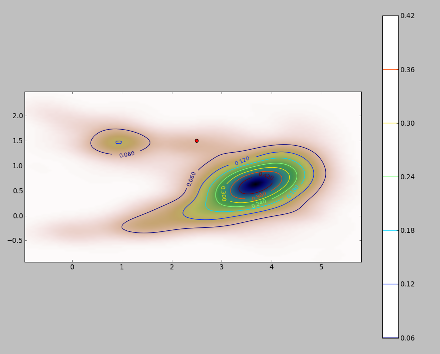
The PDF of my 2D data set (obtained through python's stats.gaussian_kde module) looks like this:

enter image description here

where the red dot represents the new object $p[x_p, y_p]$ plotted over the PDF of my data set.

So the question is: how can I calculate the above integral for the limits $x, y:\hat{f}(x, y) < \hat{f}(x_p, y_p)$ when the pdf looks like that?


Add

I did some tests to see how well the Monte Carlo method I mention in one of the comments worked. This is what I got:

table

The values appear to vary a bit more for lower density areas with both bandwidths showing more or less the same variation. The largest variation in the table occurs for the point (x,y)=(2.4,1.5) comparing Silverman's 2500 vs 1000 sample value, which gives a difference of 0.0126 or ~1.3%. In my case this would be largely acceptable.

Edit: I just noticed that in 2 dimension Scott's rule is equivalent to Silverman's according to the definition given here.

$\endgroup$
8
  • 2
    $\begingroup$ Have you noticed your estimator is not unimodal, but that the recommendation you are following explicitly applies only to "unimodal" distributions? That doesn't mean you're doing something wrong, but it should generate some hard thinking about what the answer might mean. $\endgroup$
    – whuber
    Commented Jul 5, 2013 at 15:49
  • $\begingroup$ Hi @whuber, actually the answer in that question says that it is "well behaved" for unimodal distributions, so I thought that perhaps it could work on my problem with some modification. Does "well behaved" mean "works only" in statistical jargon (honest question)? Cheers. $\endgroup$
    – Gabriel
    Commented Jul 5, 2013 at 16:07
  • $\begingroup$ My main concern is that the KDE may be sensitive to the choice of bandwidth and I expect your integral, especially for marginal places like that shown in the illustration, will be very sensitive to the choice. (The calculation itself, by the way, is easy once you have created a raster image like this: it is proportional to the average value in the image among points whose value is less than that of the "probe" point.) You can approach this by computing the answer for a full range of reasonable bandwidths and see whether it changes in any material way within that range. If not, you're fine. $\endgroup$
    – whuber
    Commented Jul 26, 2013 at 21:26
  • $\begingroup$ I won't comment on the solution, but the integration can be done by simple Monte Carlo: sample points from $\hat{f}$ (that's easy, since the kde is a mixture of densities that are easy to sample from), and count the fraction of points that fall inside the integration region (where the inequality holds). $\endgroup$
    – Zen
    Commented Jul 27, 2013 at 1:06
  • $\begingroup$ How many observations do you have in your dataset? $\endgroup$
    – Hong Ooi
    Commented Jul 27, 2013 at 6:16

2 Answers 2

13
$\begingroup$

A simple way is to rasterize the domain of integration and compute a discrete approximation to the integral.

There are some things to watch out for:

  1. Make sure to cover more than the extent of the points: you need to include all locations where the kernel density estimate will have any appreciable values. This means you need to expand the extent of the points by three to four times the kernel bandwidth (for a Gaussian kernel).

  2. The result will vary somewhat with the resolution of the raster. The resolution needs to be a small fraction of the bandwidth. Because the calculation time is proportional to the number of cells in the raster, it takes almost no extra time to perform a series of calculations using coarser resolutions than the intended one: check that the results for the coarser ones are converging on the result for the finest resolution. If they are not, a finer resolution may be needed.

Here is an illustration for a dataset of 256 points:
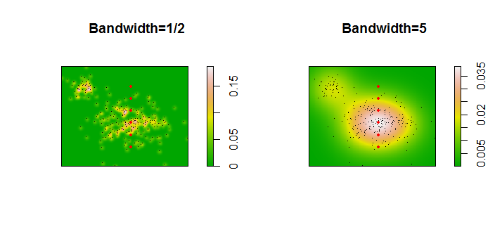
Figure 1

The points are shown as black dots superimposed on two kernel density estimates. The six large red points are "probes" at which the algorithm is evaluated. This has been done for four bandwidths (a default between 1.8 (vertically) and 3 (horizontally), 1/2, 1, and 5 units) at a resolution of 1000 by 1000 cells. The following scatterplot matrix shows how strongly the results depend on bandwidth for these six probe points, which cover a wide range of densities:
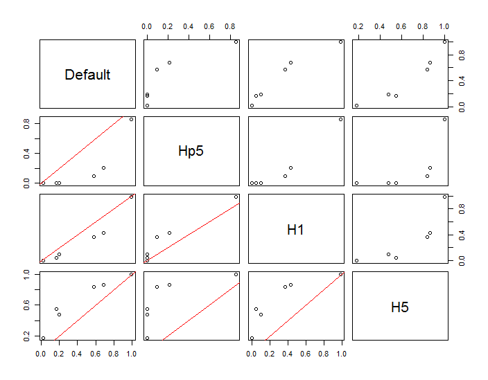
Figure 2

The variation occurs for two reasons. Obviously the density estimates differ, introducing one form of variation. More importantly, the differences in density estimates can create large differences at any single ("probe") point. The latter variation is greatest around the medium-density "fringes" of clusters of points--exactly those locations where this calculation is likely to be used the most.

This demonstrates the need for substantial caution in using and interpreting the results of these calculations, because they can be so sensitive to a relatively arbitrary decision (the bandwidth to use).


R Code

The algorithm is contained in the half dozen lines of the first function, f. To illustrate its use, the rest of the code generates the preceding figures.

library(MASS)     # kde2d
library(spatstat) # im class
f <- function(xy, n, x, y, ...) {
  #
  # Estimate the total where the density does not exceed that at (x,y).
  #
  # `xy` is a 2 by ... array of points.
  # `n`  specifies the numbers of rows and columns to use.
  # `x` and `y` are coordinates of "probe" points.
  # `...` is passed on to `kde2d`.
  #
  # Returns a list:
  #   image:    a raster of the kernel density
  #   integral: the estimates at the probe points.
  #   density:  the estimated densities at the probe points.
  #
  xy.kde <- kde2d(xy[1,], xy[2,], n=n, ...)
  xy.im <- im(t(xy.kde$z), xcol=xy.kde$x, yrow=xy.kde$y) # Allows interpolation $
  z <- interp.im(xy.im, x, y)                            # Densities at the probe points
  c.0 <- sum(xy.kde$z)                                   # Normalization factor $
  i <- sapply(z, function(a) sum(xy.kde$z[xy.kde$z < a])) / c.0
  return(list(image=xy.im, integral=i, density=z))
}
#
# Generate data.
#
n <- 256
set.seed(17)
xy <- matrix(c(rnorm(k <- ceiling(2*n * 0.8), mean=c(6,3), sd=c(3/2, 1)), 
               rnorm(2*n-k, mean=c(2,6), sd=1/2)), nrow=2)
#
# Example of using `f`.
#
y.probe <- 1:6
x.probe <- rep(6, length(y.probe))
lims <- c(min(xy[1,])-15, max(xy[1,])+15, min(xy[2,])-15, max(xy[2,]+15))
ex <- f(xy, 200, x.probe, y.probe, lim=lims)
ex$density; ex$integral
#
# Compare the effects of raster resolution and bandwidth.
#
res <- c(8, 40, 200, 1000)
system.time(
  est.0 <- sapply(res, 
           function(i) f(xy, i, x.probe, y.probe, lims=lims)$integral))
est.0
system.time(
  est.1 <- sapply(res, 
           function(i) f(xy, i, x.probe, y.probe, h=1, lims=lims)$integral))
est.1
system.time(
  est.2 <- sapply(res, 
           function(i) f(xy, i, x.probe, y.probe, h=1/2, lims=lims)$integral))
est.2
system.time(
  est.3 <- sapply(res, 
           function(i) f(xy, i, x.probe, y.probe, h=5, lims=lims)$integral))
est.3
results <- data.frame(Default=est.0[,4], Hp5=est.2[,4], 
                      H1=est.1[,4], H5=est.3[,4])
#
# Compare the integrals at the highest resolution.
#
par(mfrow=c(1,1))
panel <- function(x, y, ...) {
  points(x, y)
  abline(c(0,1), col="Red")
}
pairs(results, lower.panel=panel)
#
# Display two of the density estimates, the data, and the probe points.
#
par(mfrow=c(1,2))
xy.im <- f(xy, 200, x.probe, y.probe, h=0.5)$image
plot(xy.im, main="Bandwidth=1/2", col=terrain.colors(256))
points(t(xy), pch=".", col="Black")
points(x.probe, y.probe, pch=19, col="Red", cex=.5)
xy.im <- f(xy, 200, x.probe, y.probe, h=5)$image
plot(xy.im, main="Bandwidth=5", col=terrain.colors(256))
points(t(xy), pch=".", col="Black")
points(x.probe, y.probe, pch=19, col="Red", cex=.5)
$\endgroup$
6
  • $\begingroup$ Amazing answer, although I'm not sure I understand the meaning of the Default and Hp5 bandwidths (I assume H1 and H5 mean h=1 and h=5) Is Hp5 the value h=1/2? If so what is Default? $\endgroup$
    – Gabriel
    Commented Jul 29, 2013 at 21:07
  • 1
    $\begingroup$ Your understanding is correct. ("p5" means ".5".) The default is computed automatically by kde2d using bandwidth.nrd. For the sample data it equals $3$ in the horizontal direction and $1.85$ in the vertical direction, roughly halfway between the values of $1$ and $5$ in the test. Notice that these default bandwidths are large enough to place an appreciable proportion of the total density well beyond the extent of the points themselves, which is why that extent needs to be expanded regardless of what integration algorithm you might choose to use. $\endgroup$
    – whuber
    Commented Jul 29, 2013 at 21:17
  • $\begingroup$ So am I understanding correctly if I say that as I increase the bandwidth used the extent of the resulting kde also increases (and so I need to extend the integration limits)? Given that I can live with an error of <10% in the resulting value of the integral, what do you think about using Scott's rule? $\endgroup$
    – Gabriel
    Commented Jul 29, 2013 at 21:36
  • $\begingroup$ I think that because these rules were developed for entirely different objectives, you should suspect they might not perform well for your purposes, especially if it is to implement a suggestion made at stats.stackexchange.com/questions/63263. It is premature to be worrying about whose rule of thumb you might use for the KDE; at this stage you should be seriously concerned whether the entire approach will even work reliably. $\endgroup$
    – whuber
    Commented Jul 29, 2013 at 21:40
  • 1
    $\begingroup$ Scratch the above. I do have a way of knowing if the implementation is working and even of quantifying how well it is working. It's a bit complicated and time consuming but I can (should be able to) do it. $\endgroup$
    – Gabriel
    Commented Jul 29, 2013 at 21:47
1
$\begingroup$

If you have a decent number of observations, you may not need to do any integration at all. Say your new point is ${\bf{x}}_0$. Assume you have a density estimator $\hat f$; sum up the number of observations ${\bf{x}}$ for which $\hat f({\bf{x}}) < \hat f({\bf{x}}_0)$ and divide by the sample size. This gives you an approximation to the required probability.

This assumes that $\hat f({\bf{x}}_0)$ is not "too small" and your sample size is large enough (and spread-out enough) to give a decent estimate in the low-density regions. 20000 cases does seem large enough though, for bivariate ${\bf{x}}$.

$\endgroup$
1
  • $\begingroup$ Some quantitative analysis of this recommendation, or at least one example of an actual application, would be welcome. I suspect that the accuracy of your proposal is heavily dependent on the shape of the kernel. This would make me reluctant to rely on such a calculation without substantial study of its properties. $\endgroup$
    – whuber
    Commented Jul 29, 2013 at 18:27

Your Answer

By clicking “Post Your Answer”, you agree to our terms of service and acknowledge you have read our privacy policy.

Not the answer you're looking for? Browse other questions tagged or ask your own question.