3
$\begingroup$

I obtained two sets of data from a Monte Carlo simulation of polymer movement.

One is a list of $r^2_{end-to-end}$,

#r-end-squared
58617.14512069625
55606.1082220041
51244.724846185505
65344.140277928964
63392.17236605068
62101.375689808614
58814.8832777033
60040.00627213609
52019.130880313125
56984.44642212785
... ... ... ... ...

and another is a list of $\overrightarrow{r}_{end-to-end}$

#   r_end-X     r_end-Y    r_end-Z
-177.236 100.309 -130.930
-184.354 88.047 -117.760
-172.577 87.168 -117.745
-197.651 103.270 -124.953
-190.053 104.223 -128.100
-187.985 102.387 -127.593
-190.839 91.210 -118.643
-193.851 98.069 -113.333
-177.084 83.960 -116.667
-178.312 92.759 -128.782
... ... ... ... ...

The autocorrelation formula used in the case of $r^2_{end-to-end}$ is as follows:

$$ R(t) = \frac{1}{(n - t) \cdot \sigma^2} \sum_{i=0}^{n-t-1} (X_i - \mu)(X_{i+t} - \mu) $$

where:

  • $( n )$ is the number of observations in the dataset,
  • $( t )$ is the lag, or the distance between the compared points,
  • $( \mu )$ is the mean of the dataset,
  • $( \sigma^2 )$ is the variance of the dataset,
  • $( X_i )$ and $( X_{i+t} )$ are the data points at indexes $( i )$ and $( i+t )$ respectively.

The autocorrelation value $( R(t) )$ for each lag $( t )$ is calculated by summing the product of the mean-adjusted data points separated by the lag, and then normalizing the sum by dividing it by the product of the variance and the number of terms in the sum (adjusted for the lag). This calculation is done for each lag from 0 up to the specified number of lags (numLag), but not exceeding the number of data points (n). The computed autocorrelation values are then filtered based on the specified thresholds (thresholdMin and thresholdMax).


Here's how I adapted the autocorrelation function for the vector dataset:

  1. Calculate the mean vector $\boldsymbol{\mu}$ by averaging each component of the vectors separately:

$$ \boldsymbol{\mu} = \left( \frac{1}{n}\sum_{i=0}^{n-1} x_i, \frac{1}{n}\sum_{i=0}^{n-1} y_i, \frac{1}{n}\sum_{i=0}^{n-1} z_i \right) $$

  1. Calculate the autocorrelation function for the vector dataset using the dot product to get a scalar autocorrelation value for each lag $t$:

$$ R(t) = \frac{1}{(n - t) \cdot \sigma^2} \sum_{i=0}^{n-t-1} \left( \mathbf{X}_i - \boldsymbol{\mu} \right) \cdot \left( \mathbf{X}_{i+t} - \boldsymbol{\mu} \right) $$

where $\mathbf{X}_i$ is the vector at index $i$, and $\sigma^2$ is the variance of the magnitude squared of the end-to-end distance vectors. The variance in this case can be calculated as:

$$ \sigma^2 = \frac{1}{n} \sum_{i=0}^{n-1} \left( \| \mathbf{X}_i - \boldsymbol{\mu} \|^2 \right) - \left( \| \boldsymbol{\mu} \|^2 \right) $$

Here, $\| \mathbf{X}_i - \boldsymbol{\mu} \|^2$ is the squared magnitude of the vector difference $\mathbf{X}_i - \boldsymbol{\mu}$.

In the autocorrelation function, the dot product in the summands will give us a scalar value, as the dot product of two vectors is a scalar. This is appropriate since I am interested in the correlation of the scalar magnitudes of the end-to-end vectors.

Now, the correction to the formula is in how $\sigma^2$ is interpreted. In the scalar case, this is simply the variance of the dataset, but for vectors, you're dealing with magnitudes, so you need to find the average of the squared distances from the mean vector, as shown above.


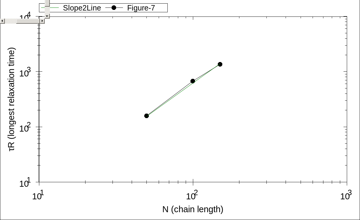
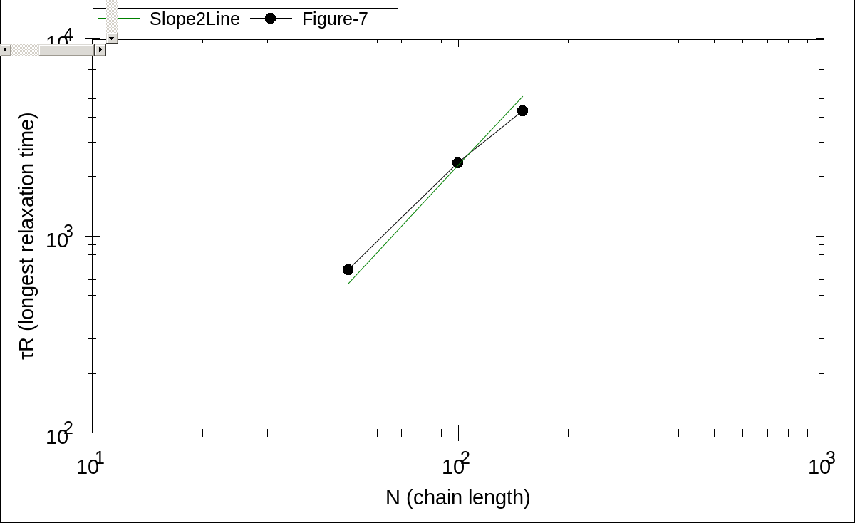
Both formulas were used for an exponential-decay $y = A0 * Exp(-x * 1/t0)$ curve fitting and then drawing a plot for polymer length vs. tau.

The autocorrelation formula used in the case of $r^2_{end-to-end}$ is working fine and giving plots as expected.

enter image description here

However, the formula used in the case of $\overrightarrow{r}_{end-to-end}$ is not giving similar plots.

enter image description here

So, what am I missing in the vector case?

$\endgroup$
13
  • 1
    $\begingroup$ Could you explain what you are trying to do. Fitting an exponential decay curve? To what decay data? Computing autocorrelation? Of what time series? Obtain best fit values? Based on what method? $\endgroup$ Commented Feb 7 at 10:25
  • $\begingroup$ @SextusEmpiricus, Check the edit. $\endgroup$
    – user366312
    Commented Feb 8 at 11:51
  • $\begingroup$ I understand, I think, the following: You have a time series of 3D vector and you are computing two autocorrelation functions, $\rho_1(t)$ and $\rho_2(t)$ for this. One is based on a radial squared distance $r^2$, the other is based on the sum of the autocorrelations for the three seperate coordinates... $\endgroup$ Commented Feb 8 at 12:43
  • $\begingroup$ ... What I don't understand is “Both formulas were used for an exponential-decay...”. 1) How where they used for this and what does $\tau R$ mean in the plots. Is this some value obtained from the autocorrelation functions? 2) Also, you have 'chain length' on the horizontal axis... does this mean that you did this for several different polymers and are investigating some change in the autocorrelation as function of properties of those different polymers? 3) In addition I don't understand what the filtering is doing. $\endgroup$ Commented Feb 8 at 12:46
  • $\begingroup$ And 4) what's the matter with the graphs? You are asking whether you are missing something, but why do you think that you are missing something? $\endgroup$ Commented Feb 8 at 12:48

2 Answers 2

1
+100
$\begingroup$

If your time series is a random walk like a type of Brownian motion, then the distance from the starting point is not a stationary time series, and an autocorrelation function has little meaning.

In the comments you referred to an article CMST 22(4) 179-185 (2016). They use the term autocorrelation function, but that appears to be more like the mean square displacement. While in that article this was defined as an average $MSD = \left< (r(t) -r(0))^2 \right>$, it might be possible that they used a rolling average $MSD = \left< (r(s+t) -r(s))^2 \right>$. An autocorrelation function is also a rolling average, but of the correlation, and not of a difference.

So it seems that what you are doing with autocorrelation functions is not the same, and it may be a cause for the unexpected difference that you observe in your model fits. The use of an autocorrelation function for the distance time series is already unclear, this is even more the case for the correlation defined for vectors. There is little reason to believe that this should give similar results as the article.

$\endgroup$
3
$\begingroup$

I have not seen any packages or functions that automate the whole process. So, you may have to create your own procedures. First, we need to ensure whether the spreadsheet has the displacement records or position records and whether the autocorrelation is for displacement or position. Next, we follow answer to "Python - How to find a correlation between two vectors?" https://stackoverflow.com/questions/3045040/python-how-to-find-a-correlation-between-two-vectors by finding the cosine of the angle between the two vectors, which requires dot products and vector magnitudes (norm) and equals the correlation coefficient. See the relationship between the quantities at https://en.wikipedia.org/wiki/Dot_product#Geometric_definition. Last, fit an exponential decay of the autocorrelation-coefficient series following https://douglas-watson.github.io/post/2018-09_exponential_curve_fitting/.

In summary, the procedure is

library(dplyr)
tribble(
       ~ x,     ~ y,      ~ z,
  -177.236, 100.309, -130.930,
  -184.354,  88.047, -117.760,
  -172.577,  87.168, -117.745,
  -197.651, 103.270, -124.953,
  -190.053, 104.223, -128.100,
  -187.985, 102.387, -127.593,
  -190.839,  91.210, -118.643,
  -193.851,  98.069, -113.333,
  -177.084,  83.960, -116.667,
  -178.312,  92.759, -128.782) %>% 
  {slice(., -1) - slice(., -nrow(.))} %>%
  mutate(
    dot = x[1] * x + y[1] * y + z[1] * z, 
    norm = sqrt(x^2 + y^2 + z^2), 
    cosine = dot/(norm[1] * norm)
  )
"       x       y       z         dot      norm      cosine
1  -7.118 -12.262  13.170  374.471468 19.351265  1.00000000
2  11.777  -0.879   0.015  -72.852838 11.809767 -0.31878346
3 -25.074  16.102  -7.208 -113.895352 30.658362 -0.19197633
4   7.598   0.953  -3.147 -107.214240  8.278975 -0.66921636
5   2.068  -1.836   0.507   14.470198  2.811507  0.26596593
6  -2.854 -11.177   8.950  275.238646 14.600450  0.97416787
7  -3.012   6.859   5.310    7.267058  9.182272  0.04089772
8  16.767 -14.109  -3.334    9.748272 22.165553  0.02272687
9  -1.228   8.799 -12.115 -258.706984 15.023435 -0.88987608"

Without differencing rows, I found that the autocorrelation is very close to one.

tribble(
       ~ x,     ~ y,      ~ z,
  -177.236, 100.309, -130.930,
  -184.354,  88.047, -117.760,
  -172.577,  87.168, -117.745,
  -197.651, 103.270, -124.953,
  -190.053, 104.223, -128.100,
  -187.985, 102.387, -127.593,
  -190.839,  91.210, -118.643,
  -193.851,  98.069, -113.333,
  -177.084,  83.960, -116.667,
  -178.312,  92.759, -128.782) %>% 
  {slice(., -1) - slice(., -nrow(.))} %>%
  mutate(
    dot = x[1] * x + y[1] * y + z[1] * z, 
    norm = sqrt(x^2 + y^2 + z^2), 
    cosine = dot/(norm[1] * norm)
  )
"      x     y     z    dot  norm cosine
   <dbl> <dbl> <dbl>  <dbl> <dbl>  <dbl>
 1 -177. 100.  -131. 58617.  242.  1    
 2 -184.  88.0 -118. 56924.  236.  0.997
 3 -173.  87.2 -118. 54747.  226.  0.999
 4 -198. 103.  -125. 61750.  256.  0.998
 5 -190. 104.  -128. 60911.  252.  0.999
 6 -188. 102.  -128. 60294.  249.  0.999
 7 -191.  91.2 -119. 58507.  243.  0.996
 8 -194.  98.1 -113. 59033.  245.  0.995
 9 -177.  84.0 -117. 55083.  228.  0.998
10 -178.  92.8 -129. 57769.  239.  1.00 "

Neither of the autocorrelation coefficients align with an exponential curve.

$\endgroup$
8
  • $\begingroup$ This answer is incorrect. $\endgroup$
    – user366312
    Commented Feb 7 at 17:08
  • $\begingroup$ @user366312, why exactly? $\endgroup$ Commented Feb 8 at 9:31
  • 1
    $\begingroup$ @user366312, but this is not what your question says. You should have included such information in the question before putting up a bounty. Now a user made the effort of writing an answer but you are not happy with it because of the additional conditions that you have omitted. The target should not be redrawn once a shooting competition has begun. $\endgroup$ Commented Feb 8 at 10:23
  • 1
    $\begingroup$ @user366312, that seems like a different reason that you gave the first time. Moreover, I do not see where he says it is not possible. He does say it does not align, but you could always find the best fit, regardless of how bad that fit happens to be. But I am not sure if he provides the method for fitting or stops before that. $\endgroup$ Commented Feb 8 at 11:09
  • 1
    $\begingroup$ @user366312, I do not mean to make you do anything. Sorry if my inquiries might have come across that way. I wished to clarify why the answer was inadequate and what your question actually is, and I think we got to the bottom of it (more or less). I hope our exchange will help other users tailor their answers to address you problem in the best possible way. $\endgroup$ Commented Feb 8 at 11:49

Your Answer

By clicking “Post Your Answer”, you agree to our terms of service and acknowledge you have read our privacy policy.

Not the answer you're looking for? Browse other questions tagged or ask your own question.